6 Measures of Central Tendency
Measures of central tendency are numerical indicators that describe a “typical” observation within a data set. These measures help summarize data and provide insight into the distribution. The three most commonly used central measures are:
- Mean (Arithmetic Average): The sum of all observations divided by the number of observations, representing the “balance point” of the distribution.
- Median: The middle value when observations are arranged in ascending order.
- Mode: The most frequently occurring value in the data set.
We will use the follwing running example in this chapter.
Example 6.1: Income
We have income data (in thousands of €) for 18 individuals:
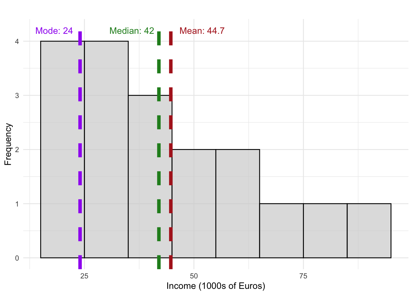
20 22 24 24 26 27 30 34 40 44 45 47 55 57 60 75 85 90We will in the following show how we compute each of the shown measure of central tendency in the follwing.
We will see that for this example, the median income is the most representative value, as it is less affected by high-income extreme values.
6.1 Arithmetic Mean
The mean is calculated by summing all values and dividing by the number of observations. It is often used as a measure of central tendency because it incorporates all data points, making it a valuable summary statistic. However, the mean is sensitive to outliers, meaning that extreme values can pull it higher or lower, potentially misrepresenting the typical value in a skewed distribution. Despite this, in normally distributed data, the mean is a reliable and widely used indicator of the data set’s center.
The mean is calculated differently depending on whether we are working with an entire population or a sample: For a population, the mean (\(\mu\), just a fancy Greek way of saying “the mean of \(X\)”) is given by: \[ \mu = \frac{\sum_{i=1}^{N} x_i}{N} \]
where \(N\) is the population size. For a sample, the mean (\(\bar{x}\)) is an estimate of \(\mu\) and is calculated as: \[ \bar{x} = \frac{\sum_{i=1}^{n} x_i}{n} \] where \(n\) is the sample size.
Example 6.1: Income
The mean income is: \[\bar{x} = \frac{20 + 22 + 24 + 24 + \cdots + 85 + 90}{18} = 44.7 \] Thus, the mean income is 44 700 €.
6.2 Median
The median is the middle value of a dataset when arranged in ascending order. It represents the point where half of the observations are below and half are above, making it a useful measure of central tendency for skewed distributions. Unlike the mean, the median is not affected by outliers, making it a more robust indicator of typical values in cases where extreme values exist. For example, in income data, the median often provides a better reflection of the typical salary than the mean, which can be skewed by very high incomes. If there is an even number of observations, the median is the average of the two middle values. The median position is found using: \[ \frac{n + 1}{2} \]
Example 6.1: Income
For our sorted income data we get that the median is located at the position \[ \frac{19}{2} = 9.5 \] The median is then the average of the 9th and 10th values (40 and 44):** \[ \frac{40 + 44}{2} =42 \] Thus, the median income is 42 000 €.
6.3 Mode
The mode is the most frequently occurring value in a data set. A data set can have one mode (unimodal), multiple modes (multimodal), or no mode at all if all values are unique. The mode is particularly useful for categorical data, such as identifying the most popular product in a sales dataset or the most common salary range in a workforce. In a histogram, the mode corresponds to the peak of the distribution, highlighting where data points concentrate the most.
Example 6.1: Income
The most frequently occurring values in the income example is 24.
6.4 Which Measure Should You Choose?
The appropriate measure of central tendency depends on the data type:
| Data Type | Suitable Measure(s) |
|---|---|
| Nominal Data (categories) | Mode |
| Ordinal Data (ranked categories) | Mode, Median |
| Interval Data (e.g., temperature) | Mode, Median, Mean |
| Ratio Data (e.g., income, weight) | Mode, Median, Mean |
When deciding between the mean and median, the mean is preferred for normally distributed data without outliers, while the median is better suited for skewed distributions or data sets with extreme values since it is not influenced by outliers. The mode, while useful for categorical and multimodal data, may not always provide meaningful insights in numerical data sets.
In our example, the median income (42 thousand euros) is a better representation of a “typical” income than the mean (44.7 thousand euros) due to high-income values skewing the mean upward.