19 Central Limit Theorem
Imagine you’re running around collecting sample means; one sample here, another there, all from the same population. At first, your collection looks messy: skewed, bumpy, unpredictable. But as your sample size grows, something magical happens. No matter how weird or wonky the original data is, the distribution of your sample means starts to smooth out. And before long, it begins to look suspiciously bell-shaped; that’s the Central Limit Theorem at work. It tells us that if your sample size is large enough, the sampling distribution of the mean will be approximately normal, with a mean equal to the population mean and a standard deviation (called the standard error) that shrinks as \(n\) grows. This makes it the statistical superhero behind confidence intervals, hypothesis tests, and your ability to make meaningful conclusions from messy real-world data.
19.1 A Universal Pattern
Up until now, we’ve seen that when the population distribution is normal, the sampling distribution of the mean \(\bar{X}\) is also normally distributed, regardless of sample size. But what happens when the population isn’t normally distributed at all?
This is where the Central Limit Theorem (CLT) enters like the hero of probability theory. It answers the following question:
What does the sampling distribution of \(\bar{X}\) look like if the population itself is not normal?
The short answer: approximately normal, as long as the sample size is large enough. The CLT intuitively states: If we take a large enough random sample of size \(n\) from any population (with finite mean \(\mu\) and variance \(\sigma^2\)), then the sampling distribution of the sample mean \(\bar{X}\) will be approximately normal: \[\bar{X} \sim \mathcal{N} \left( \mu, \frac{\sigma^2}{n} \right)\]
This approximation becomes better as \(n\) increases. But what does large enough actually mean? There’s no hard rule, but a common rule of thumb is that \(n \geq 30\) is usually sufficient, especially if the population distribution is moderately skewed. For extremely skewed or heavy-tailed distributions, a larger sample may be needed for the approximation to hold well. A visual inspection of the distribution may therefore be necessary to determine if normal approximation is appropriate.
One of the most powerful outcomes of the Central Limit Theorem is that it allows us to approximate probabilities involving the sample mean \(\bar{X}\), even when we do not know the distribution of the population, as long as the sample size \(n\) is sufficiently large.
Suppose we want to compute the probability: \[ P(\bar{X} \leq c) \]
where \(c\) is some value. Thanks to the CLT, we can standardize the sample mean and relate this probability to the standard normal distribution:
\[ P(\bar{X} \leq c) \approx P\left(Z \leq \frac{c - \mu_{\bar{X}}}{\sigma_{\bar{X}}} \right) \]
Since \(\bar{X}\) has mean \(\mu_X\) and standard deviation \(\sigma_X / \sqrt{n}\), we substitute:
\[ P(\bar{X} \leq c) \approx P\left(Z \leq \frac{c - \mu_X}{\sigma_X / \sqrt{n}} \right) \]
where
-
\(\mu_X\): population mean
-
\(\sigma_X\): population standard deviation
-
\(n\): sample size
- \(Z\): standard normal variable
This approximation is foundational in statistics. It simplifies problems involving averages and enables the use of standard normal tables or software tools to answer probability questions.
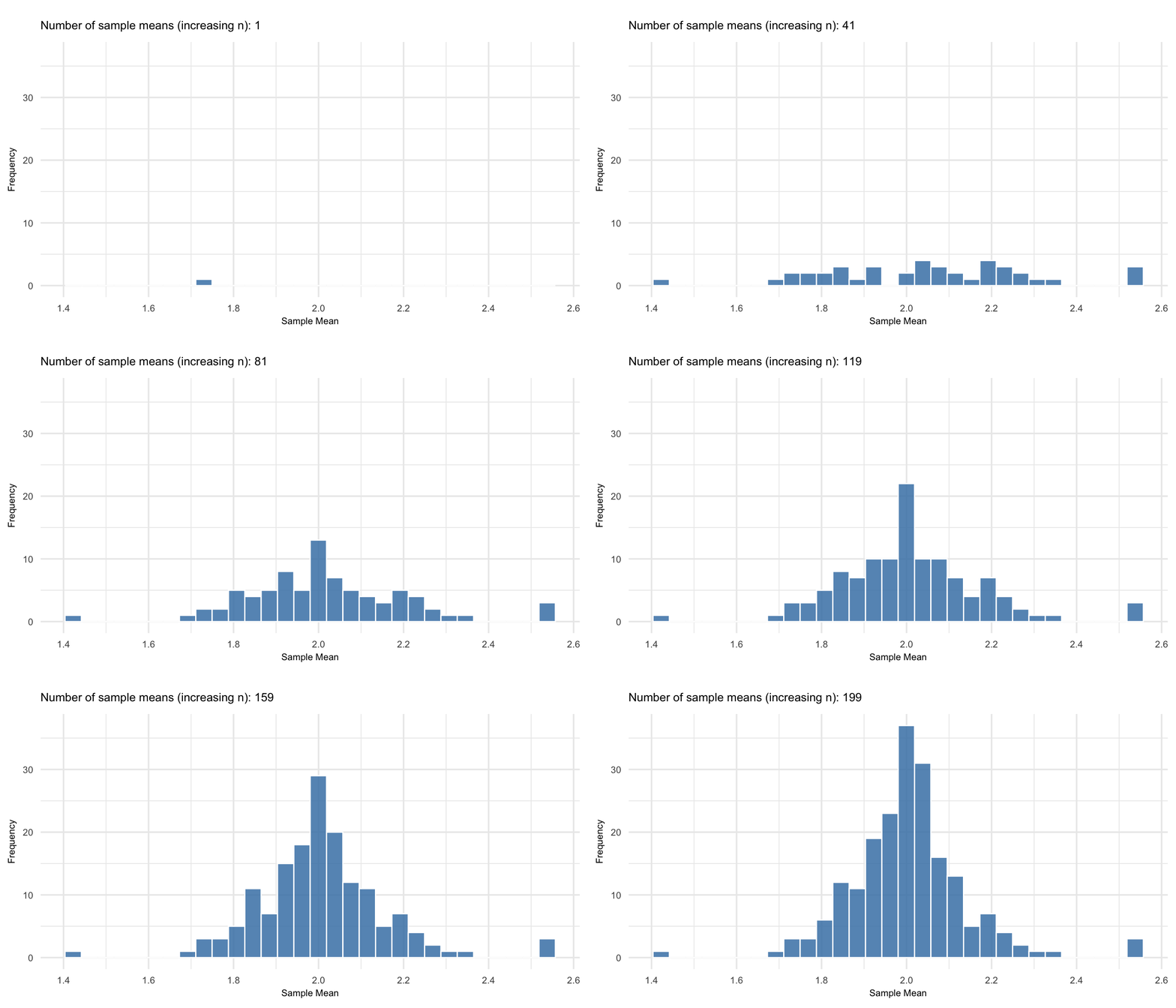
Figure 19.1 show an animation on how the distribution of sample means evolves as we draw one sample from increasingly larger sample sizes from a highly skewed population (chi-squared with 2 degrees of freedom). As the number of sample means accumulates, and as each mean is based on more data, the distribution of those means becomes increasingly symmetric and bell-shaped; demonstrating the Central Limit Theorem in action. Even though the original population is far from normal, the sample means tend toward a normal distribution as \(n\) increases.
19.2 The Formal Statement of CLT
Let \(X_1, X_2, \dots, X_n\) be a sequence of independent and identically distributed (i.i.d.) random variables with:
- Mean: \(\mu = E(X_i)\)
- Variance: \(\sigma^2 = \operatorname{Var}(X_i) < \infty\)
Define the sample mean:
\[ \bar{X}_n = \frac{1}{n} \sum_{i=1}^n X_i \]
Then the Central Limit Theorem states:
\[ \frac{\bar{X}_n - \mu}{\sigma / \sqrt{n}} \xrightarrow{d} \mathcal{N}(0, 1) \quad \text{as } n \to \infty \]
In words: As the sample size increases, the standardized sample mean converges in distribution to a standard normal distribution, regardless of the shape of the original distribution (as long as the mean and variance are finite).
The proof of this theorem is rather long and beyond the scope of this course.
Example 19.1: Applying the CLT
Suppose we draw a random sample of size \(n = 100\) from a population with:
- Mean \(\mu = 65\)
- Variance \(\sigma^2 = 64\)
What is the probability that the sample mean \(\bar{X}\) is less than 63?
From the CLT, since \(n \geq 30\), we can assume: \[ \bar{X} \sim \mathcal{N}\left(65, \frac{64}{100}\right) = \mathcal{N}(65, 0.64) \]
We want to calculate: \[ P(\bar{X} \leq 63) \]
We standardize the sample mean: \[ Z = \frac{63 - 65}{\sqrt{0.64}} = \frac{-2}{0.8} = -2.5 \]
and find \[ P(\bar{X} \leq 63) = P(Z \leq -2.5) \]
Using the standard normal distribution (Appendix A): \[ P(Z \leq -2.5) = 1 - P(Z \leq 2.5) = 1 - 0.994 = 0.006 \]