14 Continuous Probability Distributions
Until now, we have mainly worked with discrete random variables, meaning variables that can only take on a finite or countably infinite number of possible values. For instance, the number of heads when tossing coins or the number of defective items in a sample are all discrete.
However, not all random phenomena can be described in this way. A continuous random variable is a variable that can take on any value within an interval on the real number line. Rather than jumping between isolated values, a continuous variable can assume an infinite continuum of possible outcomes.
Because a continuous random variable can take any value within an interval, it is practically impossible to guess the exact value that a randomly selected observation will have. In fact, the probability that the variable exactly equals any specific value is zero. Consequently, for continuous random variables, we do not measure probabilities at single points. Instead, we consider the probability that the variable falls within a given interval.
To handle continuous random variables, we develop continuous analogues of the probability mass functions used for discrete variables. These continuous probability distributions are described using probability density functions, which allow us to calculate the probability that the variable lies within a specified range.
To summarize visually:
| Feature | Discrete Random Variable | Continuous Random Variable |
|---|---|---|
| Possible values | Finite or countable infinite set (e.g., 0, 1, 2, …) | Any real number within an interval (e.g., [0, 1]) |
| Probability at a single point | Positive (e.g., \(P(X = 2) > 0\)) | Always zero (\(P(X = 2) = 0\)) |
| Probability distribution type | Probability mass function (PMF) | Probability density function (PDF) |
| How probabilities are calculated | Sum over points (\(\sum\)) | Integrate over intervals (\(\int\)) |
In discrete settings, probabilities are assigned to individual points. For continuous random variables, we instead measure the “area under the curve” of the density function across an interval.
As we move forward, we will develop the tools needed to work with continuous distributions, starting with probability density functions and moving toward important continuous models such as the uniform and normal distributions.
14.1 Probability Density Function (PDF)
A continuous random variable can take on all possible values within some interval on the real number line. The interval may be bounded or extend to infinity in one or both directions.
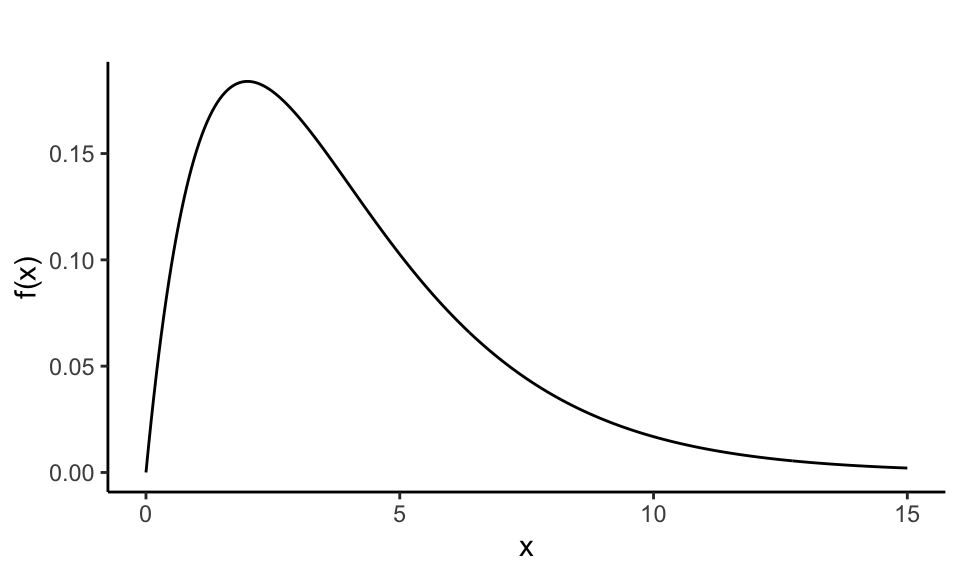
The probability distribution of a continuous random variable \(X\) is described by a so-called probability density function \(f(x)\). The density function represents how the values of \(X\) are distributed across the real line.
A typical shape of a probability density function might look like the following:
In contrast to discrete random variables, continuous variables do not assign positive probability to specific points. Instead, the probability that \(X\) falls within a particular interval \([a, b]\) is given by the area under the curve of the density function between \(a\) and \(b\):
\[ P(a \leq X \leq b) = \text{area under } f(x) \text{ from } a \text{ to } b \]
The properties that every valid probability density function must satisfy are: - \(f(x) \geq 0\) for all \(x\) (the function must be non-negative everywhere) - The total area under \(f(x)\) over the entire real line equals 1:
\[ \int_{-\infty}^{\infty} f(x) , dx = 1 \]
This ensures that the random variable must take on some value in the real numbers with total probability one.
We can also visually highlight the probability over a specific interval by shading the area between two points \(a\) and \(b\):
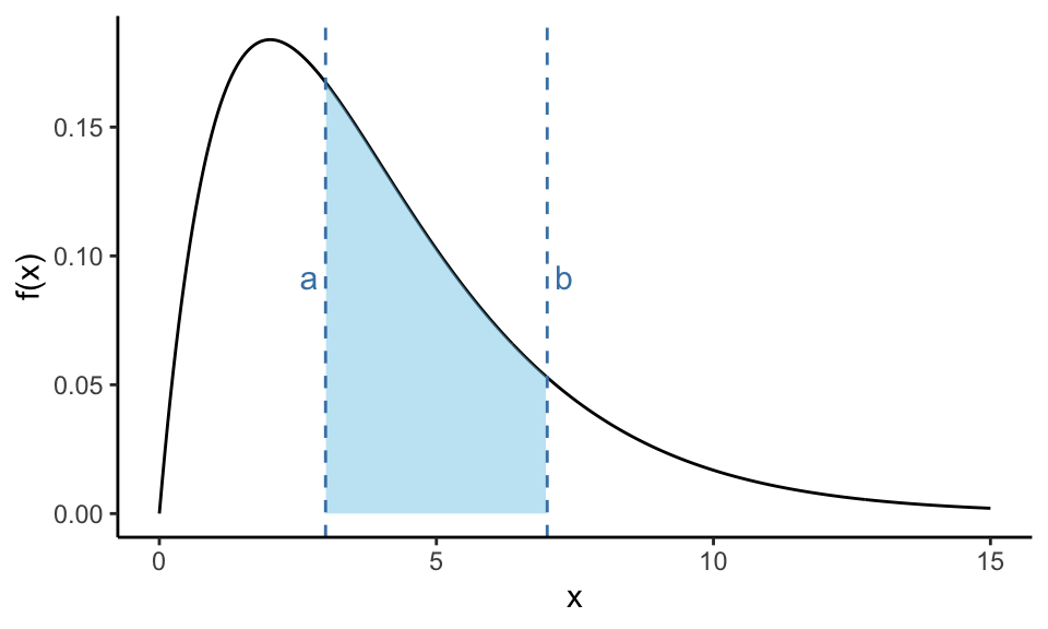
In this plot, the shaded area between \(a = 3\) and \(b = 7\) represents \(P(3 \leq X \leq 7)\); the probability that the random variable falls within this interval.
This concept, relating probabilities to areas under a curve, is a fundamental idea when working with continuous random variables, and it distinguishes them clearly from the discrete case where we sum probabilities at isolated points.
When working with continuous random variables, we are always interested in the probability that a value falls within an interval, never at a single point. This is because the area under the curve at a single value is zero, which means:
\[ P(X = a) = 0 \]
Whether we specify the interval as open, closed, or half-open does not affect the probability. For example, the following expressions are all equivalent:
\[ P(a \leq X \leq b) = P(a \leq X < b) = P(a < X \leq b) = P(a < X < b) \]
They all describe the same shaded region under the curve between \(a\) and \(b\).
Formally, the probability that \(X\) falls within an interval \([a, b]\) is given by integrating the probability density function:
\[ P(a \leq X \leq b) = \int_a^b f(x) \, dx \]
However, in this course, we do not require formal calculations using integrals.
We can work with the cumulative distribution function (CDF), which is defined as:
\[ F(x) = P(X \leq x) \]
This function gives the total probability accumulated up to the value \(x\), that is, the area under the density curve from the lower bound of the distribution up to \(x\).
Using the CDF, we can express interval probabilities as the difference of cumulative values:
\[ P(a \leq X \leq b) = P(X \leq b) - P(X \leq a) = F(b) - F(a) \]
This relationship is especially useful when we don’t have access to the density function itself but can look up or compute values of the cumulative distribution. It also reinforces the idea that probability for continuous variables is tied to the area between two points, not the height at a point.
14.2 Expectation and Variance for Continuous Variables
Just as we did with discrete random variables, we can define the expected value and variance for continuous random variables. These two quantities serve as important measures of central tendency and spread, respectively.
The expected value of a continuous random variable \(X\) with density function \(f(x)\) is given by:
\[ E(X) = \mu_X = \int_{-\infty}^{\infty} x f(x) \, dx \]
This can be interpreted as a kind of weighted average, where the values of \(x\) are weighted by their relative likelihood; in this case, the density function \(f(x)\).
The variance is defined as:
\[ \operatorname{Var}(X) = \sigma_X^2 = \int_{-\infty}^{\infty} (x - \mu)^2 f(x) \, dx \]
Just like in the discrete case, this measures how spread out the values of \(X\) are around the mean \(\mu\).
Intuitively, the expected value can be thought of as the balance point of the distribution, the point at which the density function would balance perfectly if it were a physical object. The variance, as before, describes how tightly or widely the values of \(X\) tend to cluster around this center.
14.3 The Normal Distribution
Among all continuous probability distributions, none is more important or more widely used than the normal distribution. This may seem strange, since very few real-world quantities are exactly normally distributed. Nevertheless, the normal distribution plays a central role in probability theory and statistics, especially as a powerful approximation tool.
Mathematically, a random variable \(X\) is said to follow a normal distribution if its probability density function is given by:
\[ f(x) = \frac{1}{\sigma \sqrt{2\pi}} \, e^{- \frac{1}{2} \left( \frac{x - \mu}{\sigma} \right)^2}, \quad \text{for } -\infty < x < \infty \]
We denote this by writing:
\[ X \sim \mathcal{N}(\mu, \sigma) \]
Here, \(\mu\) is the mean of the distribution, and \(\sigma^2\) is the variance (with \(\sigma\) being the standard deviation).
This density function has a characteristic bell shape: it is symmetric about the mean \(\mu\), and the spread of the curve is determined by \(\sigma\). The larger the value of \(\sigma\), the more spread out the distribution becomes.
Despite its somewhat complicated appearance, the normal distribution is incredibly useful because many phenomena in practice, especially sums and averages of random variables, tend to follow a distribution that closely resembles the normal. This fact is supported by the central limit theorem, which guarantees that under mild conditions, the sum of a large number of independent random variables tends toward a normal distribution, regardless of the original distributions. We will return to this in more details later.
Moreover, the probabilities associated with the normal distribution have already been computed and tabulated. These tables allow us to quickly look up values without performing integrals manually, making the normal distribution not only powerful in theory but also very practical in application.
It is this combination of mathematical elegance, approximation power, and computational convenience that explains the normal distribution’s central role in both theoretical and applied statistics.
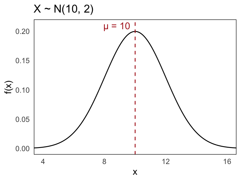
Let us now look at a concrete example. Suppose \(X\) is a normally distributed random variable with mean \(\mu = 10\) and standard deviation \(\sigma = 2\):
\[ X \sim \mathcal{N}(10, 2) \]
The density function of \(X\) is bell-shaped and symmetric around the mean, with most of its probability mass concentrated within a few standard deviations from the center.
Below is the probability density function for this distribution:
In practice, there are a few key characteristics of the normal distribution that are particularly important to understand.
First, the shape of the normal distribution is completely determined by two parameters: the mean \(\mu\) and the standard deviation \(\sigma\). These control the center and the spread of the distribution, respectively.
The sample space of a normal distribution is the entire real number line, meaning that the variable can take on any real value, both positive and negative.
Graphically, the density function of a normal distribution always has the same bell-shaped curve, regardless of the specific values of \(\mu\) and \(\sigma\). The mean \(\mu\) determines the central location of the curve, while the standard deviation \(\sigma\) determines how wide or narrow the curve appears.
A key feature of the normal distribution is that it is symmetric around the mean \(\mu\). This symmetry implies that probabilities on either side of the mean are equal for equally sized intervals. In addition, as \(x \to \pm\infty\), the density function \(f(x)\) approaches zero, meaning that extremely large or small values are increasingly unlikely, but not impossible.
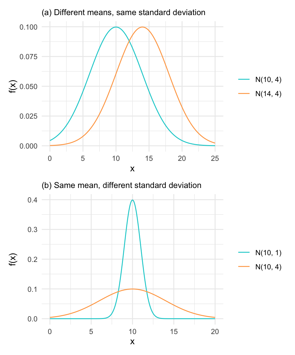
The shape of a normal distribution is fully determined by its mean \(\mu\) and standard deviation \(\sigma\). Changing either of these parameters modifies the appearance of the distribution in predictable ways. This is shown in Figure 14.1.
In (a), we compare two normal distributions with different means but the same standard deviation. This results in curves with identical shapes, but centered at different locations. Shifting \(\mu\) translates the curve horizontally without altering its height or spread.
In (b), we hold the mean constant and vary the standard deviation. This causes the curve to either compress or stretch. A smaller \(\sigma\) yields a sharper, narrower peak, while a larger \(\sigma\) produces a flatter, wider distribution.
But first, we will learn how to calculate probabilities using normal distribution tables.
14.3.1 Area under curve
When using a normal distribution curve to model probability, the logic is as follows: we want to determine the probability that a randomly selected individual falls within a certain interval, say \((a, b)\). This is equivalent to finding the proportion of individuals in the population whose values lie between \(a\) and \(b\).
In a normal distribution, this probability corresponds to the area under the curve between \(a\) and \(b\). Since the total area under the entire curve is equal to 1 (or 100%), the shaded region gives us the desired probability.
This relationship between area and probability allows us to calculate how likely it is to observe values within specific ranges, and by symmetry, how unusual values far from the mean are.
Let us visualize this with the previously mentioned empirical rule in Figure 7.3, which summarizes how the area is distributed across standard deviations from the mean. This is shown in Figure 14.2.
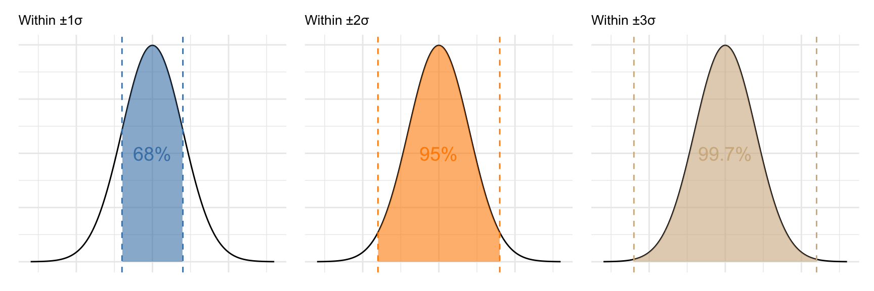
In practice, the most important takeaway is this:
- Approximately 68% of values lie within one standard deviation from the mean (\(\mu \pm \sigma\))
- About 95% lie within two standard deviations (\(\mu \pm 2\sigma\))
- Nearly 99.7% lie within three standard deviations (\(\mu \pm 3\sigma\))
This is known as the empirical rule, and it forms the basis for many practical applications of the normal distribution. It also shows that values far from the mean are rare, making them candidates for being considered “unusual” or outliers in statistical reasoning.
14.4 The Standard Normal Distribution
In practice, the values for which we want to calculate probabilities do not always align with the specific values shown in a table. Fortunately, thanks to the properties of the normal distribution, we don’t need a separate table for every possible mean and standard deviation.
Instead, we make use of a powerful idea: that any normal distribution can be converted into a standard normal distribution, and this makes calculating probabilities far simpler.
The standard normal distribution is the special case where the mean is 0 and the standard deviation is 1. That is:
\[ Z \sim \mathcal{N}(0, 1) \]
This is our reference distribution. Because it measures distances in units of standard deviation from the mean, we can interpret a value like \(z = 1.5\) as “1.5 standard deviations above the mean”.
Since the normal distribution is symmetric around the mean, values less than 0 represent outcomes below average, and values greater than 0 are above average. Below is the standard normal curve:
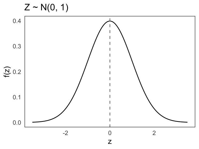
The plot shows the familiar bell shape, now centered at 0. By using the standard normal distribution, we only need to consult a single probability table, shown in Appendix A, to find probabilities for a wide range of problems. The transformation is done through standardization, which we’ll explore in the next section.
We denote the cumulative probability function of the standard normal by \(F(z)\) or \(P(Z \leq z)\), and for values of \(z\) between 0.00 and 3.00, these values are commonly found in standard Z-tables. Because of symmetry, we can compute probabilities for both tails of the distribution (and for negative values of \(z\)), i.e.
\[ P(Z \leq -z) = 1 - P(Z \leq z) \]
This is the foundation for calculating probabilities with normal distributions; we convert our variable to a Z-score and then read the probability directly from this reference distribution.
Example 14.1: Standard Normal Distribution
Let \(Z \sim \mathcal{N}(0,1)\) be a standard normal variable. We’ll now walk through several examples of calculating probabilities using the standard normal distribution, visualizing the corresponding areas under the curve in each case.
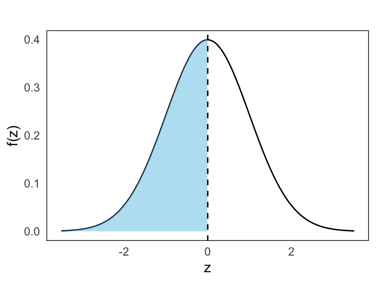
- \(P(Z \leq 0)\)
By symmetry, the probability that \(Z\) is less than or equal to 0 is:
\[ P(Z \leq 0) = F(0) = 0.5 \]
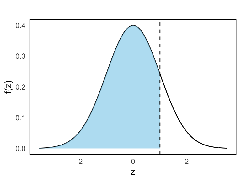
- \(P(Z \leq 1)\)
We use the standard normal table:
\[ P(Z \leq 1) = F(1) = 0.8413 \]
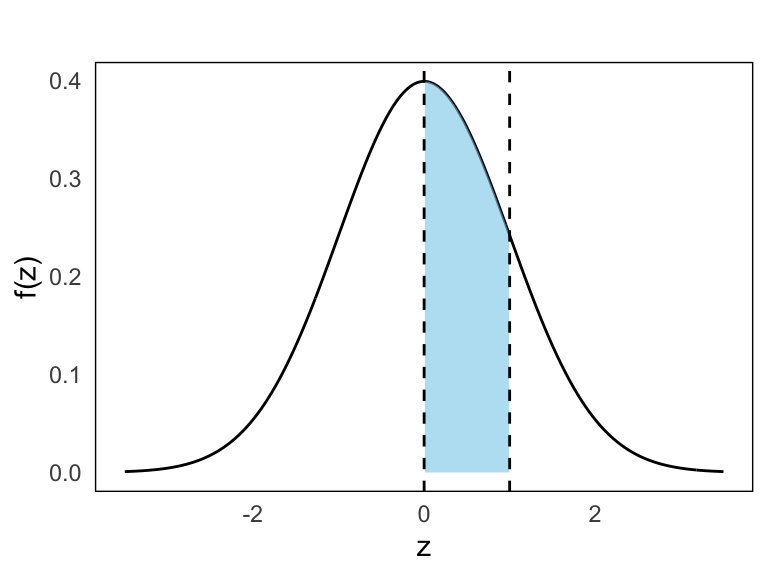
- \(P(0 \leq Z \leq 1)\)
This is the difference between two cumulative probabilities:
\[ P(0 \leq Z \leq 1) = F(1) - F(0) = 0.8413 - 0.5000 = 0.3413 \]
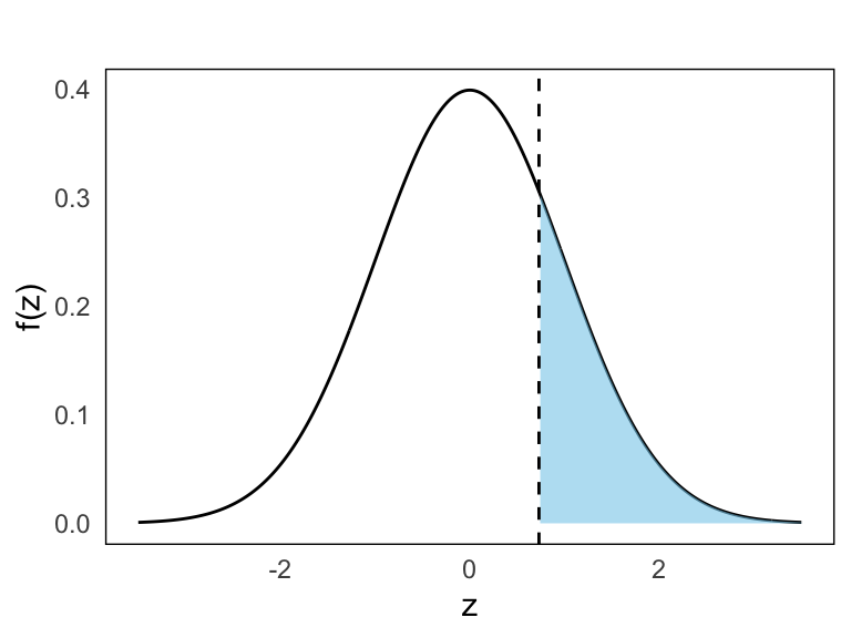
- \(P(Z \geq 0.73)\)
We use the complement rule:
\[ P(Z \geq 0.73) = 1 - P(Z \leq 0.73) = 1 - 0.7673 = 0.2327 \]
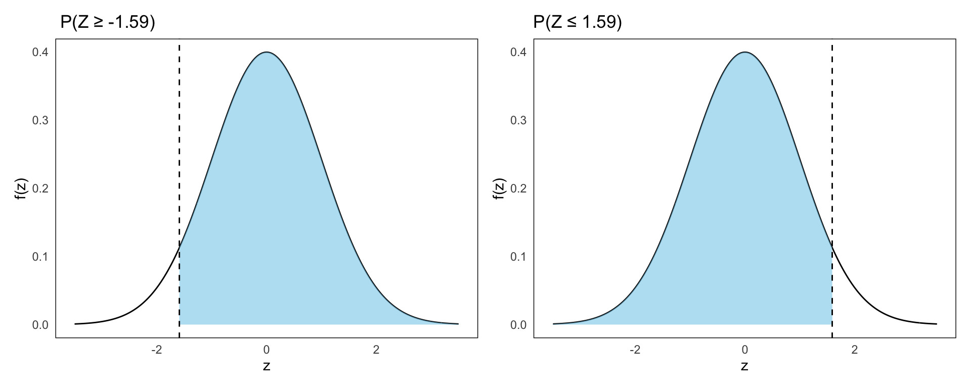
- \(P(Z \geq -1.59)\)
Using symmetry:
\[ P(Z \geq -1.59) = P(Z \leq 1.59) = F(1.59) = 0.9441 \]
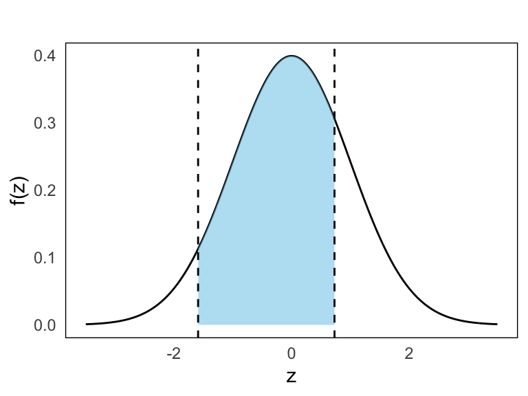
- \(P(-1.59 \leq Z \leq 0.73)\)
We combine cumulative values:
\[ \begin{split} P(-1.59 \leq Z \leq 0.73) & = F(0.73) - (1 - F(1.59)) \\ & = 0.7673 - (1 - 0.9441) \\ & = 0.7114 \end{split} \]
14.5 From Normal to Standard Normal Distribution
Suppose a random variable \(X\) follows a normal distribution with mean \(\mu\) and standard deviation \(\sigma\), written:
\[ X \sim \mathcal{N}(\mu, \sigma) \]
We often want to compute the probability \(P(X \leq x)\) for some value \(x\). While this can’t be calculated directly from \(X\) without integration, we can convert the problem to one involving the standard normal distribution using the transformation:
\[ Z = \frac{X - \mu}{\sigma} \]
This transformation maps \(X\) to a standard normal variable \(Z \sim \mathcal{N}(0,1)\). The beauty of this is that we can now use our standard normal table in Appendix A to calculate:
\[ P(X \leq x) = P\left(Z \leq \frac{x - \mu}{\sigma} \right) \]
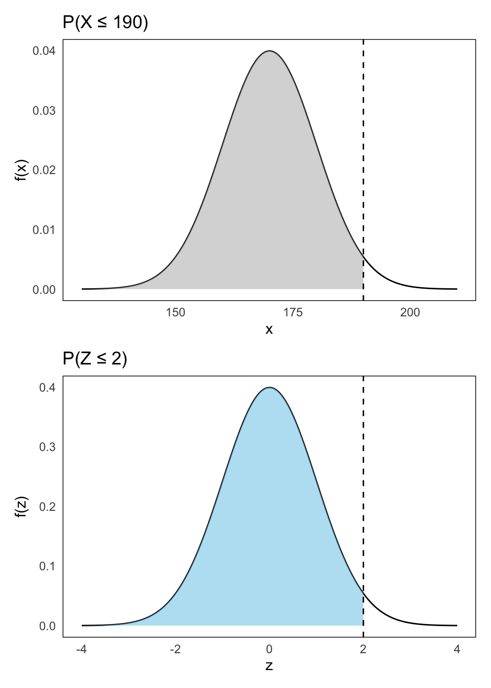
Example 14.2: \(X \sim \mathcal{N}(170, 10)\)
We want to compute:
- \(P(X \leq 190)\)
We begin by standardizing:
\[ Z = \frac{X - 170}{10}, \quad \text{so} \quad \frac{190 - 170}{10} = 2 \]
Then use the standard normal table to find the correpsondign probability area:
\[ P(X \leq 190) = P(Z \leq 2) = 0.9772 \]
This is shown below in Figure 14.3 where both shaded areas are exactly the same.
14.6 Normal Approximation to the Binomial Distribution
As hinted before, one of the normal distribution’s greatest superpowers is its flexibility; it’s like the Swiss Army knife of probability! Why? Because it can be used to approximate probabilities in many important situations, especially when working with other discrete distributions.
As seen in Figure 14.4, the binomial distribution becomes increasingly symmetric and bell-shaped as the sample size grows. When the number of trials is large enough, the distribution of a binomially distributed variable begins to closely resemble that of a normal distribution. In such cases, it becomes not only possible but also practical to use the normal distribution as an approximation.
The normal approximation is particularly helpful when exact binomial probabilities are cumbersome to calculate.
14.6.1 When can we approximate?
A common rule of thumb is:
\[ np(1 - p) > 5 \]
If this condition is met, the binomial distribution can be reasonably approximated by a normal distribution that shares the same mean and variance.
14.6.2 How is the approximation performed?
Well, suppose \(X \sim \text{Bin}(n, p)\) and the above condition is satisfied. Then we can approximate \(X\) using a normal distribution:
\[ X \overset{\text{apx}}{\sim} \mathcal{N}(\mu, \sigma) \]
where
\[ \mu = E(X) = np \quad \text{and} \qquad \sigma = \sqrt{\operatorname{Var}(X)} = \sqrt{np(1 - p)} \]
To compute a probability such as \(P(X \leq c)\), where \(c\) is an integer, we use the standard normal distribution:
\[ P(X \leq c) \approx P\left(Z \leq \frac{c - \mu}{\sigma} \right) \]
This gives us an approximate value by translating the binomial question into a standard normal one.
Example 14.3: Binomial to Normal
Let \(X \sim \text{Bin}(44, 0.45)\). We wish to approximate the probability:
\[ P(X \leq 26) \]
First, compute the mean and variance of \(X\):
\[ E(X) = 44 \cdot 0.45 = 19.8 \\ \operatorname{Var}(X) = 44 \cdot 0.45 \cdot 0.55 = 10.89 \]
Since \(nP(1 - P) = 10.89 > 5\), the normal approximation is applicable.
Now standardize:
\[ Z = \frac{26 - 19.8}{\sqrt{10.89}} \approx \frac{6.2}{3.3} \approx 1.88 \]
Using the standard normal distribution:
\[ P(X \leq 26) \approx P(Z \leq 1.88) = 0.9699 \]
For comparison, the exact binomial value is:
\[ P(X \leq 26) = 0.9786 \]
So the normal approximation is quite close, especially useful when exact computation is difficult.
14.6.3 Continuity Correction
When using a normal distribution to approximate a binomial, it’s important to remember that we are replacing a discrete distribution (which only takes whole number values) with a continuous one (which takes all real values). To improve the accuracy of this approximation, we use a technique called the continuity correction.
The idea is simple: when we compute a probability such as \(P(X \leq c)\) for a binomial variable, we approximate it not with \(P(Z \leq z)\) but with a slightly adjusted value:
\[ P(X \leq c) \approx P\left(Z \leq \frac{c + 0.5 - \mu}{\sigma} \right) \]
The addition of \(0.5\) shifts the cutoff slightly to the right, accounting for the fact that we’re now working with an area under a continuous curve rather than summing discrete spikes.
Example 14.3: Binomial to Normal (cont’d)
Recall from earlier that:
\[ X \sim \text{Bin}(44, 0.45), \quad \mu = 19.8, \quad \sigma = \sqrt{10.89} \approx 3.3 \]
We want to compute:
\[ P(X \leq 26) \]
Using the continuity correction, we calculate:
\[ P(X \leq 26) \approx P\left(Z \leq \frac{26 + 0.5 - 19.8}{3.3} \right) = P(Z \leq 2.0) = 0.9772 \]
This is a better approximation than the earlier uncorrected value of \(P(Z \leq 1.88) = 0.9699\).
The table below summarizes and compraes the results:
| Value | |
|---|---|
| Exact binomial | 0.9786 |
| Normal approximation | 0.9699 |
| With continuity correction | 0.9772 |
As shown above, the continuity correction significantly improves the accuracy of the approximation and is highly recommended when using the normal distribution to approximate binomial probabilities.
Exercises
- Suppose human reaction times to a specific stimulus are normally distributed with a mean of 300 milliseconds and a standard deviation of 50 milliseconds. You randomly select one person. What is the probability that their reaction time is between 237.5 ms and 325 ms?
Solution
We standardize both endpoints:
\[ Z_1 = \frac{237.5 - 300}{50} = -1.25 \quad\text{and}\quad Z_2 = \frac{325 - 300}{50} = 0.5 \]
From the standard normal table:
- \(P(Z \leq 0.5) = 0.6915\)
- \(P(Z \leq -1.25) = 0.1056\)
So:
\[ P(237.5 \leq X \leq 325) = 0.6915 - 0.1056 = \boxed{0.5859} \]
This means there’s about a 59% chance a person reacts within this interval.
- An economic survey estimates that 35% of a certain population is underemployed. In a sample of 100 individuals, let \(X\) be the number who are underemployed. What is the probability that at most 42 people are underemployed? Use the normal approximation with continuity correction.
Solution
We model \(X \sim \text{Bin}(100, 0.35)\)
- Mean: \(\mu = 100 \cdot 0.35 = 35\)
- Standard deviation: \(\sigma = \sqrt{100 \cdot 0.35 \cdot 0.65} = \sqrt{22.75} \approx 4.77\)
Using continuity correction:
\[ P(X \leq 42) \approx P\left(Z \leq \frac{42 + 0.5 - 35}{4.77} \right) = P(Z \leq 1.57) \]
From Z-table:
\[ P(Z \leq 1.57) = \boxed{0.9418} \]
So there’s a 94% chance that 42 or fewer people in the sample are underemployed.
- In a national voter turnout study, the probability that an eligible person votes is estimated to be 65%. Suppose a researcher surveys 200 randomly selected citizens. Let \(X\) be the number of individuals in the sample who actually voted. What is the probability that between 120 and 140 people (inclusive) voted, using a normal approximation with continuity correction?
Solution
We model \(X \sim \text{Bin}(n = 200, p = 0.65)\).
- Mean: \(\mu = 200 \cdot 0.65 = 130\)
- Standard deviation: \(\sigma = \sqrt{200 \cdot 0.65 \cdot 0.35} = \sqrt{45.5} \approx 6.74\)
We apply continuity correction to the bounds:
- Lower bound: \(X = 120 \Rightarrow Z = \frac{119.5 - 130}{6.74} \approx -1.56\)
- Upper bound: \(X = 140 \Rightarrow Z = \frac{140.5 - 130}{6.74} \approx 1.56\)
So:
\[ P(120 \leq X \leq 140) \approx P(-1.56 \leq Z \leq 1.56) \]
From standard normal tables:
- \(P(Z \leq 1.56) = 0.9406\)
- \(P(Z \leq -1.56) = 1 - 0.9406 = 0.0594\)
Therefore:
\[ P(-1.56 \leq Z \leq 1.56) = 0.9406 - 0.0594 = \boxed{0.8812} \]
There’s an 88.1% chance that between 120 and 140 people in the sample voted.