28 Multiple Linear Regression

In earlier chapters, we worked with simple linear regression, where we modeled a response variable $y$ using a single explanatory variable $x$. However, many real-world problems involve several factors that may simultaneously influence the outcome.

Multiple linear regression extends the simple linear model by allowing more than one explanatory variable. In this framework, the goal is to model a dependent variable $y$ as a linear function of $K$ predictors:

\[ \hat{y} = b_0 + b_1 x_1 + b_2 x_2 + \dots + b_K x_K \]

Each coefficient $b_k$ represents the partial effect of predictor $x_k$ on the response, holding all other predictors constant.

Motivating Example: Smoking Type and Death Rate

To understand why multiple linear regression is often necessary, consider a classic example from Cochran (1968), which examines the relationship between smoking type and death rate.

The study compared two groups: Pipe smokers and Cigarette smokers. The outcome of interest was the death rate, measured as the number of deaths per 1,000 person-years.

Let:

$y$ be the death rate (per 1,000 person-years)
$x$ be a binary variable indicating smoking type: \[ x = \begin{cases} 0 & \text{if pipe smoker} \\ 1 & \text{if cigarette smoker} \end{cases} \]

We begin by fitting a simple linear regression model:

\[ \hat{y} = \hat{\beta}_0 + \hat{\beta}_1 x = 17 - 4x \]

Interpretation:

For pipe smokers ($x = 0$), the predicted death rate is $\hat{y} = 17$
For cigarette smokers ($x = 1$), the predicted death rate is $\hat{y} = 13$

This model seems to suggest that cigarette smokers have a lower death rate than pipe smokers by 4 deaths per 1,000 person-years. But this conclusion is counterintuitive and misleading. Why would cigarette smoking appear protective?

The likely explanation lies in confounding; in this case, the variable age. If cigarette smokers in the sample happen to be younger on average than pipe smokers, then age (a known risk factor for mortality) could explain the apparent protective effect.

To account for this, we expand the model to include age as an additional predictor:

Let:

$x_1$ = 0 for pipe smoker, 1 for cigarette smoker
$x_2$ = age (in years)

We now fit a multiple linear regression model:

\[ \hat{y} = \hat{\beta}_0 + \hat{\beta}_1 x_1 + \hat{\beta}_2 x_2 = 14 + 4x_1 + 10x_2 \]

The intercept 14 represents the baseline death rate for a pipe smoker of age 0 (not directly meaningful but needed for model structure).
The coefficient $\hat{\beta}_1 = 4$ means that, after adjusting for age, cigarette smokers have a death rate that is 4 deaths per 1,000 person-years higher than pipe smokers.
The coefficient $\hat{\beta}_2 = 10$ means that, for each additional year of age, the death rate increases by 10 deaths per 1,000 person-years, regardless of smoking type.

In the simple model, the association between smoking type and death rate appeared to suggest a protective effect of cigarette smoking. But this was due to omitting a key variable (age) which was unevenly distributed between groups.

By including age as an explanatory variable, the multiple regression model reveals the true relationship: that cigarette smoking is associated with higher mortality risk once age is accounted for.

This example highlights a critical motivation for using multiple linear regression:

to adjust for confounding factors and isolate the effect of each explanatory variable on the outcome

28.1 Data Structure for Multiple Linear Regression

In general, we work with data structured as follows: we have $n$ observations and $K$ explanatory (independent) variables. The response variable is denoted by $y$, and the predictors by $x_1, x_2, \dots, x_K$. Each row in the dataset corresponds to a single observation, and each column (aside from $y$) corresponds to one predictor.

The data can be organized in tabular form:

\[ \begin{array}{c|cccc} y & x_1 & x_2 & \cdots & x_K \\ \hline y_1 & x_{11} & x_{21} & \cdots & x_{K1} \\ y_2 & x_{12} & x_{22} & \cdots & x_{K2} \\ \vdots & \vdots & \vdots & \ddots & \vdots \\ y_n & x_{1n} & x_{2n} & \cdots & x_{Kn} \end{array} \]

This format highlights that each outcome $y_i$ is potentially influenced by all $K$ explanatory variables in the corresponding row. Our goal in multiple linear regression is to estimate how changes in each predictor $x_k$ (for $k = 1, \dots, K$) affect the response $y$, while controlling for the other predictors in the model.

28.2 Fitting the Multiple Linear Regression Model

Just as before, we use the least squares method to fit a linear function to our observed data. The goal is to model the relationship between a dependent variable $y$ and multiple explanatory variables $x_1, x_2, \dots, x_K$.

The general form of the model is:

\[ \hat{y} = b_0 + b_1 x_1 + b_2 x_2 + \cdots + b_K x_K \]

Here: - $\hat{y}$ is the predicted value of the response variable, - $b_0$ is the intercept (the expected value of $y$ when all $x_k = 0$), - $b_1, b_2, \dots, b_K$ are the estimated regression coefficients for each predictor.

Each observation $i = 1, 2, \dots, n$ contributes a data point $(y_i, x_{1i}, x_{2i}, \dots, x_{Ki})$. For each observation, we estimate:

\[ \hat{y}_i = b_0 + b_1 x_{1i} + b_2 x_{2i} + \cdots + b_K x_{Ki} \]

The coefficients $b_0, b_1, \dots, b_K$ are chosen to minimize the Error Sum of Squares (SSE), that is, the squared differences between the observed values $y_i$ and their predicted values $\hat{y}_i$:

\[ \text{SSE} = \sum_{i=1}^n (y_i - \hat{y}_i)^2 = \sum_{i=1}^n (y_i - b_0 - b_1 x_{1i} - \cdots - b_K x_{Ki})^2 \]

This minimization ensures that the fitted line (or hyperplane in higher dimensions) is as close as possible to the observed data, in the sense of minimizing prediction error.

In practice, we do not solve this minimization problem by hand. Instead, statistical software (here: R) performs the computations and returns the estimated coefficients and diagnostic statistics.

Once the least squares estimates have been obtained, we can:

Interpret the coefficients to understand the relationship between predictors and the outcome,
Predict new values of $y$ given new values of $x$,
Assess model fit using $R^2$, residual analysis, and hypothesis tests (Chapter 29).

28.3 Decomposing Variation in Multiple Linear Regression

Just like in simple linear regression, we can break down the total variation in the response variable y into two components:

\[ \sum_{i=1}^n (y_i - \bar{y})^2 = \sum_{i=1}^n (\hat{y}_i - \bar{y})^2 + \sum_{i=1}^n (y_i - \hat{y}_i)^2 \]

This identity leads to three important quantities:

SST (Total Sum of Squares): measures the total variation in y across all observations
\[ SST = \sum_{i=1}^n (y_i - \bar{y})^2 \]
SSR (Regression Sum of Squares): variation in y explained by the model
\[ SSR = \sum_{i=1}^n (\hat{y}_i - \bar{y})^2 \]
SSE (Error or Residual Sum of Squares): unexplained variation (leftover noise)
\[ SSE = \sum_{i=1}^n (y_i - \hat{y}_i)^2 \]

If the model fits the data perfectly, then all predicted values match the actual values, meaning SSE = 0. On the other hand, if none of the predictors explain any variation, then SSR = 0, and all variation remains in the residuals.

The proportion of the total variation in y that is explained by the model is measured by the coefficient of determination:

\[ R^2 = \frac{SSR}{SST} = 1 - \frac{SSE}{SST} \]

This value ranges between 0 and 1. A value near 1 indicates that the model captures most of the variation in y, while a value near 0 suggests poor explanatory power.

28.4 ANOVA Table in Multiple Regression

The ANOVA (Analysis of Variance) table breaks down and summarizes these sources of variation in a structured way:

Source	Sum of Squares (SS)	Degrees of Freedom (df)	Mean Square (MS)	F Statistic
Regression	SSR	K	$MSR = \frac{SSR}{K}$	$F = \frac{MSR}{MSE}$
Residual	SSE	$n - K - 1$	$MSE = \frac{SSE}{n - K - 1}$
Total	SST	$n - 1$

Here, K is the number of explanatory variables, and n is the number of observations.

The F-statistic in the regression row tests whether at least one of the predictors has a non-zero effect on the response variable. A large F-value indicates that the model explains a significant portion of the variation in y. We will return to this in Chapter 29.

The residual variance is the average squared error between the observed and predicted values of y. It is also referred to as the Mean Squared Error (MSE):

\[ s_e^2 = \frac{SSE}{n - K - 1} \]

A smaller residual variance implies a better-fitting model, as it indicates that the predicted values are close to the actual observations.

Example 28.1: Sales in Different Districts

To illustrate, consider a company analyzing sales performance across eight sales districts. The response variable is:

$y$: total sales (in millions of EUR)

Two potential explanatory variables are:

$x_1$: population size (in 100,000s of people)
$x_2$: advertising volume (in 10,000s of EUR)

The data from the eight districts is summarized below:

District	Sales ($y$)	Population ($x_1$)	Advertising ($x_2$)
1	5.4	5.0	5.0
2	3.8	4.2	3.0
3	10.6	10.0	9.0
4	5.2	4.4	3.5
5	4.5	3.6	5.0
6	2.7	1.3	2.0
7	2.5	2.7	1.8
8	4.5	3.0	4.7

This example raises several important questions:

How much of the variation in sales across districts can be explained by differences in population and advertising?
What is the expected change in sales if advertising increases, assuming the population remains constant?

To answer these questions, we fit a multiple linear model to the data. The model has the form:

\[ \hat{y}_i = b_0 + b_1 x_{1i} + b_2 x_{2i} + \dots + b_K x_{Ki} \]

Here: - $i = 1, 2, \dots, n$ indexes the observations (e.g., districts), - $b_0$ is the intercept, - $b_1, b_2, \dots, b_K$ are regression coefficients for each predictor, - $\hat{y}_i$ is the predicted value of $y$ for the $i$-th observation.

Below the R output from fitting this model is shown:


Call:
lm(formula = y ~ x1 + x2, data = sales_df)

Residuals:
       1        2        3        4        5        6        7        8 
-0.27273 -0.43141  0.18678  0.60826 -0.40773  0.55532 -0.30926  0.07076 

Coefficients:
            Estimate Std. Error t value Pr(>|t|)  
(Intercept)   0.4301     0.3897   1.104   0.3200  
x1            0.5464     0.1625   3.362   0.0201 *
x2            0.5021     0.1825   2.752   0.0402 *
---
Signif. codes:  0 '***' 0.001 '**' 0.01 '*' 0.05 '.' 0.1 ' ' 1

Residual standard error: 0.4981 on 5 degrees of freedom
Multiple R-squared:  0.9724,    Adjusted R-squared:  0.9614 
F-statistic:  88.1 on 2 and 5 DF,  p-value: 0.0001265

Interpretation of the Output

The regression output provides the following key pieces of information:

Estimated coefficients

Intercept ($b_0$): the predicted sales when both population and advertising are zero. Although this scenario is outside the data range, the intercept anchors the plane in the data space.
Population coefficient ($b_1$): the fitted change in sales (million EUR) for each additional 100 000 people, holding advertising constant.
Advertising coefficient ($b_2$): the fitted change in sales for each additional 10 000 EUR of advertising, holding population constant.

$R^2$$
These values show the proportion of variance in sales accounted for by the two predictors.

A typical pattern for this dataset is that both population and advertising are positively associated with sales, meaning districts with more people and larger advertising budgets tend to sell more. The multiple-regression framework allows us to state, for example:

“After adjusting for population size, an additional 10 000 EUR in advertising is associated with an estimated increase of $b_2$ million SEK in sales.”

Because the sample is small ($n=8$), coefficient estimates come with substantial uncertainty. Overall, this model demonstrates how multiple predictors jointly explain the variability in sales, and how each effect is interpreted while holding the other predictor constant; the fundamental advantage of multiple linear regression.

28.5 Adjusted R²: A Caution Against Overfitting

When fitting a multiple linear regression model, it’s tempting to keep adding explanatory variables to increase the model’s $R^2$ — the proportion of variation in the response variable explained by the model.

However, there’s a caveat:
$R^2$ can never decrease when a new variable is added to the model. Even if that variable has no real relationship with the outcome, the $R^2$ will either increase or stay the same. This means a model can appear to improve in fit simply by becoming more complex, even if the added variables contribute little or nothing meaningful.

To account for this, we use the adjusted coefficient of determination, denoted $R^2_{\text{adj}}$, which penalizes unnecessary complexity. It is defined as:

\[ R^2_{\text{adj}} = 1 - \frac{SSE / (n - K - 1)}{SST / (n - 1)} \]

where: - $SSE$ is the residual sum of squares, - $SST$ is the total sum of squares, - $n$ is the number of observations, - $K$ is the number of explanatory variables (not counting the intercept).

The adjusted $R^2$ serves as a more reliable indicator of model quality, particularly when trying out different sets of predictors. While ordinary $R^2$ always increases (or stays the same) when new variables are added, the adjusted version can decrease if the new variable does not improve the model enough to justify the increase in complexity.

This makes $R^2_{\text{adj}}$ especially useful in model selection procedures, where we experiment with different subsets of variables to find a model that balances fit and simplicity.

Note: Adjusted $R^2$ should not be interpreted as the proportion of variance explained in the same direct way as regular $R^2$. It is better viewed as a corrected measure of fit that accounts for the number of predictors.

Practical Tip

If you’re building a regression model incrementally, i.e., adding one explanatory variable at a time, keep an eye on the adjusted $R^2$. If it decreases when you add a new variable, this may signal that the variable isn’t contributing meaningfully to the model and could be excluded.

Example 28.2: Synthetic Data

We work with the constructed dataset

y	x₁	x₂
1	2	1
5	4	2
3	5	2
8	6	4
5	8	4
3	10	4
10	11	6
7	13	6

where $y$ is the outcome, $x_1$ the first predictor, and $x_2$ a second predictor.

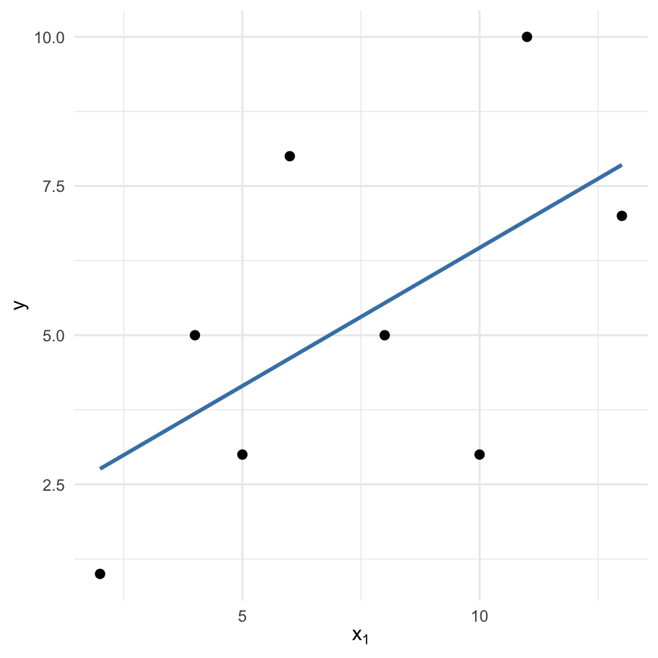
We fit a simple regression: $y$ on $x_1$, obtaining following output:


Call:
lm(formula = y ~ x1, data = df)

Residuals:
    Min      1Q  Median      3Q     Max 
-3.4656 -1.3029 -0.6971  1.7525  3.3867 

Coefficients:
            Estimate Std. Error t value Pr(>|t|)
(Intercept)   1.8348     2.1150   0.868    0.419
x1            0.4631     0.2586   1.791    0.124

Residual standard error: 2.585 on 6 degrees of freedom
Multiple R-squared:  0.3483,    Adjusted R-squared:  0.2396 
F-statistic: 3.206 on 1 and 6 DF,  p-value: 0.1236

The simple model finds a positive slope for $x_1$: higher $x_1$ values coincide with larger $y$ values. Visual inspection confirms the upward trend:

Now we fit a multiple regression: $y$ on $x_1$ and $x_2$, obtaning the following output:


Call:
lm(formula = y ~ x1 + x2, data = df)

Residuals:
       1        2        3        4        5        6        7        8 
-1.24027  1.55496  0.77724 -0.29912 -0.85457 -0.41002  0.51362 -0.04183 

Coefficients:
            Estimate Std. Error t value Pr(>|t|)   
(Intercept)   1.0355     0.8946   1.158  0.29933   
x1           -1.2223     0.3287  -3.719  0.01373 * 
x2            3.6493     0.6722   5.429  0.00287 **
---
Signif. codes:  0 '***' 0.001 '**' 0.01 '*' 0.05 '.' 0.1 ' ' 1

Residual standard error: 1.078 on 5 degrees of freedom
Multiple R-squared:  0.9055,    Adjusted R-squared:  0.8677 
F-statistic: 23.95 on 2 and 5 DF,  p-value: 0.002748

and the following plot:

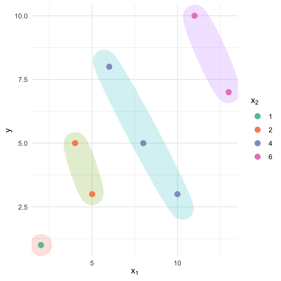
In the multiple-regression output, the sign of the coefficient on $x_1$ reverses: it becomes negative once $x_2$ is included. The scatterplot clarifies why: points with identical $x_2$ values form nearly parallel, upward-sloping bands, but across bands $x_2$ increases along with $x_1$, and $x_2$ has a much stronger positive association with $y$. That mutual rise means the simple model confounded the effect of $x_1$ with that of $x_2$; when $x_2$ is controlled for, the adjusted relationship between $x_1$ and $y$ turns negative.

This example shows how omitting a relevant variable can mislead both coefficient estimates and substantive conclusions. Multiple linear regression helps disentangle each predictor’s unique contribution by holding the others constant, preventing such reversals.

Exercises

Assume we will model (logged) hourly wage as a function of schooling and labor‐market experience and get the follwing output:


Call:
lm(formula = log(wage) ~ educ + exper, data = wage1)

Residuals:
     Min       1Q   Median       3Q      Max 
-2.05800 -0.30136 -0.04539  0.30601  1.44425 

Coefficients:
            Estimate Std. Error t value Pr(>|t|)    
(Intercept) 0.216854   0.108595   1.997   0.0464 *  
educ        0.097936   0.007622  12.848  < 2e-16 ***
exper       0.010347   0.001555   6.653 7.24e-11 ***
---
Signif. codes:  0 '***' 0.001 '**' 0.01 '*' 0.05 '.' 0.1 ' ' 1

Residual standard error: 0.4614 on 523 degrees of freedom
Multiple R-squared:  0.2493,    Adjusted R-squared:  0.2465 
F-statistic: 86.86 on 2 and 523 DF,  p-value: < 2.2e-16

Tasks

Write the estimated regression equation in the form
$\widehat{\log(\text{wage})} = b_0 + b_1 \, \text{educ} + b_2 \, \text{exper}$.
Interpret the intercept $b_0$.
Interpret $b_1$, the coefficient on educ.
Interpret $b_2$, the coefficient on exper.
Look at the output from and interpret the R-squared value reported. What does it tell us in this context?

Solution

The output gives
\[ \widehat{\log(\text{wage})} \; = \; 1.24 \; + \; 0.083\,\text{educ} \; + \; 0.019\,\text{exper} \]
Intercept ($b_0 \approx 0.217$).
A worker with zero years of schooling and zero years of experience is predicted to have $\log(\text{wage}) \approx 1.24$.
Exponentiating, that corresponds to an hourly wage of about $** 0.217**.
Although such a combination is rare, the intercept serves to anchor the regression surface.
Schooling coefficient ($b_1 \approx 0.098$).
Holding experience constant, each additional year of education is associated with an 9.8 % increase in hourly wage.
(Because the dependent variable is in logs, the coefficient can be interpreted approximately as a percentage change.)
Experience coefficient ($b_2 \approx 0.010$).
Conditional on schooling, each extra year of labor‐market experience raises predicted hourly wage by about 1.0 %.
$R^2= 0.9055$

An $R^2$ of 0.9055 means that the regression model accounts for about 90.55 % of the total variation in hourly wages observed in the sample. Put differently, differences in education and experience explain the vast majority of wage differences across individuals in this dataset, leaving only ≈ 9.45 % of the wage variation unexplained by the model.

Such a high $R^2$ suggests an excellent in-sample fit. However, we should still be cautious: a high $R^2$ does not guarantee that the model is causal, free of omitted-variable bias, or equally accurate for new data.

A researcher fits the following regression model:


Call:
lm(formula = wage ~ educ + exper + tenure, data = wage1)

Residuals:
    Min      1Q  Median      3Q     Max 
-7.6068 -1.7747 -0.6279  1.1969 14.6536 

Coefficients:
            Estimate Std. Error t value Pr(>|t|)    
(Intercept) -2.87273    0.72896  -3.941 9.22e-05 ***
educ         0.59897    0.05128  11.679  < 2e-16 ***
exper        0.02234    0.01206   1.853   0.0645 .  
tenure       0.16927    0.02164   7.820 2.93e-14 ***
---
Signif. codes:  0 '***' 0.001 '**' 0.01 '*' 0.05 '.' 0.1 ' ' 1

Residual standard error: 3.084 on 522 degrees of freedom
Multiple R-squared:  0.3064,    Adjusted R-squared:  0.3024 
F-statistic: 76.87 on 3 and 522 DF,  p-value: < 2.2e-16

In this regression of hourly wage on education, experience, and tenure, explain:

Which variables are being “controlled for” in this model?
Why is it important to control for these variables when estimating the effect of education on wages?

Solution

In this model, the variables experience and tenure are being controlled for when estimating the effect of education on wage. That means the estimated coefficient on educ reflects the relationship between education and wage, holding experience and tenure constant.
Controlling for these variables is important because they are also likely to affect wages. For example, more experienced workers usually earn higher wages, and longer tenure may also lead to higher pay. If we didn’t include these variables, the estimated effect of education might be confounded, that is, part of the variation attributed to education could actually be due to differences in experience or tenure. By including them in the regression, we isolate the effect of education net of these other factors.