Up until now, we have focused on fitting a straight line to a given dataset. This is a purely descriptive task, we are summarizing the data using a linear trend.
Now we shift our attention to statistical inference. Instead of just describing the data, we want to draw conclusions about the underlying data-generating process. In this context, we assume that the data were produced by a regression model; a hypothetical mechanism involving randomness that governs how the observed values arise.
Our concern is understanding the reliability of the coefficient estimates. Are they statistically significant? Are they meaningfully different from zero? To address such questions, we use tools like confidence intervals and hypothesis tests, just as we did in Chapter 21 and Chapter 22.
Simple Linear Regression
We think of each observed value \(y_i\) not just as a number, but as a realization of a random variable \(Y_i\), generated according to the following model:
\[
Y = \beta_0 + \beta_1 x + \varepsilon
\]
Here, \(\beta_0\) and \(\beta_1\) are unknown parameters, and \(\varepsilon\) is a random error term. This expression means that the outcome \(Y\) is made up of two parts:
- A deterministic part, which is a linear function of the predictor \(x\): \(\beta_0 + \beta_1 x\)
- A random part, the error term \(\varepsilon\), which captures the effect of other influences not included in the model
see Chapter 26 for more detail.
Assumptions
In the standard model for simple linear regression, we make the following assumptions:
The values \(x_1, x_2, \dots, x_n\) are treated as fixed, non-random inputs.
-
For each fixed \(x_i\), the corresponding response variable \(Y_i\) satisfies:
\[
Y_i = \beta_0 + \beta_1 x_i + \varepsilon_i
\]
-
The error terms \(\varepsilon_1, \varepsilon_2, \dots, \varepsilon_n\) are independent and normally distributed random variables with:
\[
\varepsilon_i \sim \mathcal{N}(0, \sigma^2)
\]
That is, they have mean 0 and the same variance \(\sigma^2\), and they are mutually independent.
Our goal is to estimate the unknown parameters \(\beta_0\) and \(\beta_1\). In practice, it is often \(\beta_1\), the slope, that is of greatest interest, as it measures the strength and direction of the relationship between \(x\) and \(y\).
To estimate these parameters, we use the least squares method, fitting a line of the form:
\[
y = b_0 + b_1 x
\]
The resulting estimates \(b_0\) and \(b_1\) are called point estimates of \(\beta_0\) and \(\beta_1\), respectively:
\[
\hat{\beta}_0 = b_0 \quad \text{and} \quad \hat{\beta}_1 = b_1
\]
Under the model assumptions, it can be shown that both \(b_0\) and \(b_1\) are unbiased estimators, meaning:
\[
E(b_0) = \beta_0 \quad \text{and} \quad E(b_1) = \beta_1
\]
Variance of the Estimator \(b_1\)
We are also interested in how precise our estimate \(b_1\) is. The variance of \(b_1\) is given by:
\[
\mathrm{Var}(b_1) = \frac{\sigma^2}{\sum (x_i - \bar{x})^2} = \frac{\sigma^2}{(n - 1)s_x^2}
\]
This tells us that the spread of the \(x\) values (captured by \(s_x^2\)) plays an important role in determining the precision of the slope estimate.
In practice, the true error variance \(\sigma^2\) is unknown. To estimate \(\mathrm{Var}(b_1)\) from the data, we replace \(\sigma^2\) with the residual variance \(s_e^2\), which is an unbiased estimator of \(\sigma^2\) and is computed as:
\[
s_e^2 = \frac{\text{SSE}}{n - 2}
\]
We then obtain the estimated variance of \(b_1\) as:
\[
s_{b_1}^2 = \frac{s_e^2}{(n - 1)s_x^2}
\]
This estimated variance will be used to construct confidence intervals and perform hypothesis tests about \(\beta_1\) in the following sections.
Confidence Interval for \(\beta_1\)
Once we have estimated the regression coefficients using the least squares method, we may want to make inferences about the true (but unknown) population parameter \(\beta_1\). Two important tools for this purpose are confidence intervals and hypothesis testing.
We already know that the point estimate \(b_1\) is an unbiased estimator of the true slope \(\beta_1\). Furthermore, under the classical linear regression assumptions (including normal, independent, and homoscedastic errors), \(b_1\) is approximately normally distributed for large samples, or t-distributed for small samples.
To quantify the uncertainty in our estimate, we construct a confidence interval for \(\beta_1\):
\[
b_1 \pm t_{\nu, \alpha/2} \cdot s_{b_1}
\]
where:
-
\(s_{b_1}\) is the estimated standard error of \(b_1\)
-
\(t_{\nu, \alpha/2}\) is the critical value from the \(t\)-distribution with \(\nu = n - 2\) degrees of freedom
-
\(\alpha\) is the significance level (e.g., \(\alpha = 0.05\) gives a 95% confidence interval)
If the sample size is large (\(n \geq 30\)), the \(t\)-distribution can be approximated by the standard normal distribution \(\mathcal{N}(0, 1)\), and the confidence interval becomes:
\[
b_1 \pm z_{\alpha/2} \cdot s_{b_1}
\]
This interval provides a range of plausible values for the true slope \(\beta_1\) at the chosen confidence level.
Hypothesis Testing for \(\beta_1\)
We may also wish to formally test hypotheses about the slope coefficient. For example, suppose we want to test whether \(\beta_1\) equals a specific value \(\beta_1^*\) (often this is 0), corresponding to the absence of a linear relationship.
We set up the null and alternative hypotheses:
-
\(H_0\): \(\beta_1 = \beta_1^*\) (null hypothesis)
-
\(H_1\): \(\beta_1 \ne \beta_1^*\) (two-sided alternative), or
-
\(H_1\): \(\beta_1 > \beta_1^*\) or \(\beta_1 < \beta_1^*\) (one-sided alternatives)
A common special case is:
-
\(H_0\): \(\beta_1 = 0\)
-
\(H_1\): \(\beta_1 \ne 0\)
This tests whether there is any linear relationship at all between the predictor and response.
To perform the test, we use the following \(t\)-statistic:
\[
t = \frac{b_1 - \beta_1^*}{s_{b_1}}
\]
If \(H_0\) is true, this statistic follows a \(t\)-distribution with \(\nu = n - 2\) degrees of freedom. In the special case when testing \(H_0: \beta_1 = 0\), the test statistic simplifies to:
\[
t = \frac{b_1}{s_{b_1}}
\]
We then compare the calculated \(t\) value to critical values from the \(t\)-distribution to decide whether to reject \(H_0\). Just like before (Chapter 22) the rejection region depends on:
- The significance level (e.g., \(\alpha = 0.05\))
- The type of alternative hypothesis (one- or two-sided)
If the \(t\)-statistic falls into the rejection region, we conclude that there is statistically significant evidence that \(\beta_1\) differs from \(\beta_1^*\) (e.g., that a linear relationship exists).
Hypothesis Testing for \(\beta_1\): t-Test and F-Test Equivalence
In simple linear regression, a common question is whether the explanatory variable \(x\) has any linear influence on the response variable \(y\). This is typically tested by assessing whether the slope coefficient \(\beta_1\) equals zero.
We state the hypotheses as:
-
\(H_0\): \(\beta_1 = 0\) (no linear relationship)
-
\(H_1\): \(\beta_1 \ne 0\) (there is a linear relationship)
To test this, we use the F-statistic from the ANOVA table, which compares the explained and unexplained variance in \(y\). We define:
-
\(F_\text{obs}\): the observed F-statistic
-
\(F_c\): the critical value from the \(F\) distribution at the chosen significance level
We reject \(H_0\) only if the observed statistic exceeds the critical value:
\[
F_{\text{obs}} > F_c
\]
In the special case of testing \(\beta_1 = 0\) in a simple linear regression**, the F-test and t-test are mathematically equivalent. That is:
\[
F = t^2
\]
Both tests always lead to exactly the same conclusion in this setting. While the t-test focuses on the slope coefficient \(b_1\) directly, the F-test evaluates the overall significance of the model. In simple linear regression, both refer to the same one predictor, so they test the same null hypothesis. We will return to the F test again below for multiple linear regression.
Example 28.1: Savings and Income
Let’s apply these ideas to an example. Suppose we want to understand how savings (in hundreds of EUR) depend on income (also in hundreds of EUR). We collect data from 10 individuals:
| 18 |
8 |
| 44 |
52 |
| 31 |
30 |
| 38 |
31 |
| 36 |
30 |
| 26 |
25 |
| 24 |
8 |
| 51 |
45 |
| 22 |
3 |
| 30 |
16 |
Our goal is to determine whether income significantly predicts savings using a simple linear regression model:
\[
y = \beta_0 + \beta_1 x + \varepsilon
\]
We’ll estimate \(b_1\), construct a confidence interval for \(\beta_1\), and test the hypothesis \(H_0: \beta_1 = 0\) using both a t-test and F-test to verify they produce the same result. This is done with R and the R output for the the above regression is as follows (the middle part is the 95% confidence interval fir \(\beta_1\)):
Call:
lm(formula = y ~ x, data = df)

Residuals:
   Min     1Q Median     3Q    Max
-7.531 -5.806 -1.435  5.764 10.077

Coefficients:
            Estimate Std. Error t value Pr(>|t|)
(Intercept) -20.8618     7.7114  -2.705 0.026852 *
x             1.4269     0.2304   6.192 0.000262 ***
---
Signif. codes:  0 '***' 0.001 '**' 0.01 '*' 0.05 '.' 0.1 ' ' 1

Residual standard error: 7.133 on 8 degrees of freedom
Multiple R-squared:  0.8274,    Adjusted R-squared:  0.8058
F-statistic: 38.34 on 1 and 8 DF,  p-value: 0.0002617
                 2.5 %    97.5 %
(Intercept) -38.644256 -3.079335
x             0.895531  1.958331
Analysis of Variance Table

Response: y
          Df  Sum Sq Mean Sq F value    Pr(>F)
x          1 1950.61 1950.61  38.343 0.0002617 ***
Residuals  8  406.99   50.87
---
Signif. codes:  0 '***' 0.001 '**' 0.01 '*' 0.05 '.' 0.1 ' ' 1
The interpretation is as follows:
- The slope coefficient \(b_1\) represents the average change in savings per 1 unit (hundred EUR) increase in income.
- The confidence interval for \(\beta_1\) tells us the range of plausible values.
- If the interval does not include 0, and the p-value is below the significance threshold (e.g., 0.05), we reject \(H_0\) and conclude that income has a statistically significant effect on savings.
- The F-statistic and the square of the t-statistic for \(b_1\) are equal, confirming the equivalence of both tests in this case.
The F-distribution arises when comparing two variances, one typically explained by a model, and the other left unexplained (the residual variance). It is commonly used in regression analysis to evaluate whether the regression model explains a significant proportion of the total variation in the response variable.
In the case of simple linear regression, the F-statistic is defined as:
\[
F = \frac{MSR}{MSE}
\]
where:
-
\(MSR\) is the mean square due to regression, i.e., the variation explained by the model,
-
\(MSE\) is the mean square error, i.e., the average of the squared residuals.
Under the null hypothesis that the slope \(\beta_1 = 0\) (no linear relationship), the F-statistic follows an F-distribution with two degrees of freedom: \((1, n - 2)\) degrees of freedom, where \(n\) is the sample size.
We use this distribution to determine whether the observed \(F\) value is unusually large. A large \(F\) value indicates that the model explains a significantly greater amount of variability than would be expected by chance.
In simple linear regression, the F-test and the squared t-test for \(\beta_1\) are mathematically equivalent: \[
F = t^2
\] However, the F-distribution plays a much larger role in multiple regression, where it tests the significance of all predictors jointly.
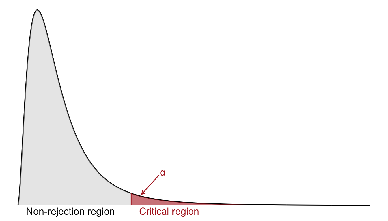
Like the chi-square test, the F-test is one-sided: we only reject the null hypothesis when the observed F-statistic is sufficiently large, as shown in Figure 29.1.
The Multiple Linear Regression Model
In multiple regression, we model the response \(y\) as a linear combination of several predictors:
\[
Y_i = \beta_0 + \beta_1 x_{1i} + \beta_2 x_{2i} + \dots + \beta_K x_{Ki} + \varepsilon_i
\]
Here:
-
\(Y_i\) is the response for observation \(i\)
-
\(x_{1i}, x_{2i}, \dots, x_{Ki}\) are the values of \(K\) predictors for observation \(i\)
-
\(\beta_0\) is the intercept
-
\(\beta_1, \dots, \beta_K\) are the unknown slope parameters
-
\(\varepsilon_i\) is the error term, capturing randomness and unobserved effects
This model allows us to assess how each predictor influences \(y\) while holding all other variables constant. In contrast to simple regression, where effects are unadjusted, multiple regression gives adjusted estimates that help untangle overlapping influences.
Assumptions and the Gauss–Markov Theorem
Like simple linear regression, the multiple linear regression model is built on a set of fundamental assumptions that ensure the reliability of the estimates and the validity of inference procedures.
At the core of the model is the assumption that the relationship between the response variable \(y\) and the explanatory variables \(x_1, x_2, \dots, x_K\) is linear in parameters. This means the model takes the form:
\[
y_i = \beta_0 + \beta_1 x_{1i} + \beta_2 x_{2i} + \dots + \beta_K x_{Ki} + \varepsilon_i,
\]
where \(\varepsilon_i\) is a random error term.
For the least squares estimates to perform well, the following assumptions must hold:
Linearity: The model must be linear in the coefficients. This does not mean that the relationship between \(x\) and \(y\) must look linear visually, but rather that the parameters appear in a linear form (i.e., no squares, logs, or interactions unless explicitly modeled).
Fixed explanatory variables: The values of the explanatory variables \(x_{1i}, \dots, x_{Ki}\) are assumed to be non-random across repeated samples. This means we condition on \(X\) when making inference about \(\beta\).
Zero mean of errors: The error terms are assumed to have an expected value of zero: \(E[\varepsilon_i] = 0\) for all \(i\).
Independence of errors: The errors are independent of one another across observations. This rules out autocorrelation or clustering unless specifically accounted for in the model.
Constant variance (Homoskedasticity): All errors have the same variance: \(\operatorname{Var}(\varepsilon_i) = \sigma^2\). If the variance of errors changes with the level of a predictor, we have heteroskedasticity, which violates this assumption.
No perfect multicollinearity: The explanatory variables must not be perfectly linearly related. That is, no predictor can be expressed as an exact linear combination of the others. This ensures that the matrix \(X'X\) is invertible.
Under these assumptions (excluding the assumption of normality) we can invoke the Gauss–Markov Theorem, which is a cornerstone of classical regression theory. It states:
Among all linear and unbiased estimators, the least squares estimator has the smallest variance. That is, it is the Best Linear Unbiased Estimator (BLUE) of the regression coefficients.
This result justifies using least squares even in the absence of normally distributed errors, as long as the other assumptions hold.
If, in addition to the above assumptions, we assume that the errors \(\varepsilon_i\) are normally distributed (i.e., \(\varepsilon_i \sim \mathcal{N}(0, \sigma^2)\)), then the least squares estimators not only remain unbiased and efficient but also follow a known sampling distribution. Specifically, the estimated coefficients follow a multivariate normal distribution, which enables us to perform t-tests, F-tests, and construct confidence intervals using standard inferential tools.
To estimate the coefficients \(\beta_0, \dots, \beta_K\), we apply the method of least squares, which minimizes the sum of squared residuals:
\[
\text{SSE} = \sum_{i=1}^n (y_i - \hat{y}_i)^2 = \sum_{i=1}^n (y_i - b_0 - b_1 x_{1i} - \dots - b_K x_{Ki})^2.
\]
The solution yields the least squares estimates \(b_0, b_1, \dots, b_K\), which are point estimates of the unknown population coefficients. Under the model assumptions, each \(b_k\) is an unbiased estimator of the corresponding \(\beta_k\):
\[
E[b_k] = \beta_k.
\]
This guarantees that the estimates are, on average, correct in repeated sampling.
In summary, the classical linear regression model provides a solid statistical framework for estimation and inference, but only when its assumptions are satisfied. The Gauss–Markov Theorem confirms the optimality of least squares under fairly minimal conditions, making it the default approach in many applied settings.
Confidence Intervals for Coefficients
Once we’ve estimated the model parameters using least squares, we often want to understand the uncertainty in those estimates. Two central tools for doing this are confidence intervals and hypothesis tests, particularly concerning individual regression coefficients. We start with the former.
Each estimated coefficient in the regression model, denoted \(b_j\), is only an estimate of the true but unknown population coefficient \(\beta_j\). Due to sampling variability, this estimate is subject to uncertainty. To capture this uncertainty, we construct a confidence interval.
A 95% confidence interval for \(\beta_j\) takes the form:
\[
b_j \pm t_{\nu, 0.025} \cdot s_{b_j}
\]
Here, \(s_{b_j}\) is the standard error of \(b_j\), and \(t_{\nu, 0.025}\) is the critical value from the \(t\)-distribution with \(\nu = n - K - 1\) degrees of freedom. The interval gives us a range of values within which the true coefficient \(\beta_j\) is likely to fall, assuming the model assumptions hold.
In practical work, these intervals are usually reported alongside the model output in software such as R, and they serve as a direct way to assess both the magnitude and uncertainty of an effect.
Hypothesis Testing for Individual Predictors
Beyond estimating coefficients, we often want to test whether a given variable contributes meaningfully to explaining \(y\) in the presence of other variables. To do this, we test whether the corresponding coefficient is equal to zero. This leads to the hypothesis:
\[
H_0: \beta_j = 0 \quad \text{versus} \quad H_1: \beta_j \neq 0
\]
We calculate a \(t\)-statistic using the formula:
\[
t = \frac{b_j}{s_{b_j}}
\]
This statistic measures how many standard errors the estimate is away from zero. If the result is far enough from zero, relative to the \(t\)-distribution, we reject the null hypothesis. The \(t\)-distribution used here has \(n - K - 1\) degrees of freedom, which accounts for both the sample size and the number of estimated parameters.
Joint Hypothesis Testing in Multiple Linear Regression
So far, we’ve looked at inference for individual regression coefficients asking whether a single explanatory variable has a statistically significant effect on the response variable. But in multiple regression, a more fundamental question often comes first:
Do all the predictors together explain any of the variation in the response variable?
This leads to a joint hypothesis test, where we test whether all regression coefficients, except the intercept, are simultaneously equal to zero. This is also knows as an omnibus test.
We formulate the hypotheses as:
\[
H_0: \beta_1 = \beta_2 = \dots = \beta_K = 0
\]
\[
H_1: \text{At least one } \beta_j \neq 0, \quad j = 1, 2, \dots, K
\]
Under the null hypothesis, none of the explanatory variables contribute linearly to explaining \(y\). In other words, we might as well discard them all and use only the intercept to predict \(y\).
To test this joint hypothesis, we use the F-statistic from the regression’s ANOVA table:
\[
F = \frac{MSR}{MSE}
\]
where:
-
\(MSR\) is the mean square for regression: \(MSR = \frac{SSR}{K}\)
-
\(MSE\) is the mean square for error: \(MSE = \frac{SSE}{n - K - 1}\)
This F-statistic follows an F-distribution with \(K\) degrees of freedom in the numerator and \(n - K - 1\) in the denominator, assuming the null hypothesis is true.
If the observed value of \(F\) is large, this suggests that the model explains a substantial portion of the variability in \(y\), and we reject the null hypothesis.
In practical terms:
- A small F-value suggests that the predictors, taken together, do not improve prediction beyond what we’d expect by chance.
- A large F-value provides evidence that at least one of the explanatory variables contributes meaningfully to the model.
Software, such as R, will compute the F-statistic and the corresponding \(p\)-value automatically. The result is typically reported in the regression output, adn the corresponding \(p\)-value can be used to perform the test,
Example 28.1: Sales in Different Districts (Cont’d)
We continue with Example 28.1 from Chapter 28 where the response variable is:
-
\(y\): total sales (in millions of EUR)
and the two explanatory variables are:
-
\(x_1\): population size (in 100,000s of people)
-
\(x_2\): advertising volume (in 10,000s of EUR)
We test (at the 1% significance level) whether \(x_1\) and \(x_2\) together can explain the variation in \(y\). In other words, we will perform an F-test.
We set up the null and alternative hypotheses as follows:
Null hypothesis: \(H_0 : \beta_1 = \beta_2 = 0\)
(Neither predictor has a linear effect on \(y\).)
Alternative hypothesis: \(H_1 :\) At least one of \(\beta_1\), \(\beta_2\) is nonzero
(At least one predictor contributes to explaining \(y\).)
We read from the output below that the observed value of the F statistic is equal to \[
F = 88.1
\] on \(K=2\) and \(n-K-1 = 8-2-1 = 5\) degrees of freedom.
Call:
lm(formula = y ~ x1 + x2, data = sales_df)

Residuals:
       1        2        3        4        5        6        7        8
-0.27273 -0.43141  0.18678  0.60826 -0.40773  0.55532 -0.30926  0.07076

Coefficients:
            Estimate Std. Error t value Pr(>|t|)
(Intercept)   0.4301     0.3897   1.104   0.3200
x1            0.5464     0.1625   3.362   0.0201 *
x2            0.5021     0.1825   2.752   0.0402 *
---
Signif. codes:  0 '***' 0.001 '**' 0.01 '*' 0.05 '.' 0.1 ' ' 1

Residual standard error: 0.4981 on 5 degrees of freedom
Multiple R-squared:  0.9724,    Adjusted R-squared:  0.9614
F-statistic:  88.1 on 2 and 5 DF,  p-value: 0.0001265
We reject the null hypothesis at the 1% significance level since the \(p\)-value is much smaller than 0.1. This means there is strong evidence that at least one of the explanatory variables has a significant linear relationship with \(y\).
In modern statistical practice, we almost always rely on the \(p\)-value reported in the regression output to evaluate the F-test. There is no need to consult critical value tables manually, since the \(p\)-value directly tells us how likely it is to observe an F-statistic as large as the one obtained, assuming the null hypothesis is true.
If the \(p\)-value is smaller than the chosen significance level (e.g., 0.05 or 0.01), we reject the null hypothesis. Otherwise, we fail to reject it. This approach is both convenient and precise, especially with software like R that handles the calculations automatically.
Exercises
- We model miles per gallon (
mpg) as a function of two predictors: horsepower (hp) and weight (wt).
Call:
lm(formula = mpg ~ hp + wt, data = mtcars)

Residuals:
   Min     1Q Median     3Q    Max
-3.941 -1.600 -0.182  1.050  5.854

Coefficients:
            Estimate Std. Error t value Pr(>|t|)
(Intercept) 37.22727    1.59879  23.285  < 2e-16 ***
hp          -0.03177    0.00903  -3.519  0.00145 **
wt          -3.87783    0.63273  -6.129 1.12e-06 ***
---
Signif. codes:  0 '***' 0.001 '**' 0.01 '*' 0.05 '.' 0.1 ' ' 1

Residual standard error: 2.593 on 29 degrees of freedom
Multiple R-squared:  0.8268,    Adjusted R-squared:  0.8148
F-statistic: 69.21 on 2 and 29 DF,  p-value: 9.109e-12
Tasks
- Write out the estimated regression equation using the model output.
- Which coefficients are statistically significant at the 5% level?
- Interpret the coefficient on
wt in the context of the model.
- What does the p-value for
hp tell you about its relationship with mpg, after controlling for wt?
- Based on the model output, we get the estimated equation:
\[
\widehat{\text{mpg}} = 37.23 - 0.032 \cdot \text{hp} - 3.88 \cdot \text{wt}
\]
- The coefficients on both
hp and wt are statistically significant at the 5% level. Their p-values are:
-
hp: p ≈ 0.002
-
wt: p < 0.001
The coefficient for wt is approximately −3.88. This means that, holding horsepower constant, a 1-unit increase in car weight (1,000 lbs) is associated with a 3.88 mpg decrease in fuel efficiency on average.
The p-value for hp (≈ 0.002) indicates that horsepower has a statistically significant negative relationship with mpg, even when we account for car weight. More horsepower reduces fuel efficiency after adjusting for weight.
- We want to understand how home prices are affected by three factors: lot size, square footage, and number of bedrooms. To do this, we fit the following multiple linear regression model using data from the
hprice1 dataset in the wooldridge package:
\[
\text{price} = \beta_0 + \beta_1\,\text{lotsize} + \beta_2\,\text{sqrft} + \beta_3\,\text{bdrms} + \varepsilon
\]
where:
-
\(\text{price}\) is the house price in thousands of dollars,
-
\(\text{lotsize}\) is the size of the lot in square feet,
-
\(\text{sqrft}\) is the size of the house in square feet,
-
\(\text{bdrms}\) is the number of bedrooms.
We obtained the following 95% confidence intervals for the estimated coefficients:
| Intercept |
\(-80.38\) |
\(36.84\) |
| lotsize |
\(0.00079\) |
\(0.00333\) |
| sqrft |
\(0.0965\) |
\(0.1491\) |
| bdrms |
\(-4.07\) |
\(31.77\) |
For each coefficient, determine whether zero is included in the interval. What does this imply about the hypothesis \(H_0: \beta_k = 0\)?
Interpret the confidence interval for \(\beta_1\) (the effect of lot size).
(a) Hypothesis Tests via Confidence Intervals:
lotsize:
The interval is \((0.00079,\; 0.00333)\), which does not contain 0.
⟶ We reject \(H_0: \beta_1 = 0\). Lot size has a statistically significant positive effect on house price.
sqrft:
The interval is \((0.0965,\; 0.1491)\), again excluding 0.
⟶ \(H_0: \beta_2 = 0\) is rejected. Square footage significantly affects price.
bdrms:
The interval is \((-4.07,\; 31.77)\), which includes 0.
⟶ We fail to reject \(H_0: \beta_3 = 0\). The number of bedrooms does not have a statistically significant effect when controlling for the other variables.
(b) Interpretation of \(\beta_1\) (lotsize):
We are 95% confident that the effect of a one square foot increase in lot size is associated with an increase in house price between $0.00079 and $0.00333 thousand dollars, or $0.79 to $3.33 dollars, holding square footage and number of bedrooms constant.