Call:
lm(formula = wage ~ female, data = wage_data)

Residuals:
    Min      1Q  Median      3Q     Max
-5.5995 -1.8495 -0.9877  1.4260 17.8805

Coefficients:
            Estimate Std. Error t value Pr(>|t|)
(Intercept)   7.0995     0.2100  33.806  < 2e-16 ***
female       -2.5118     0.3034  -8.279 1.04e-15 ***
---
Signif. codes:  0 '***' 0.001 '**' 0.01 '*' 0.05 '.' 0.1 ' ' 1

Residual standard error: 3.476 on 524 degrees of freedom
Multiple R-squared:  0.1157,    Adjusted R-squared:  0.114
F-statistic: 68.54 on 1 and 524 DF, p-value: 1.042e-1530 Categorical Variables in Regression
Up to this point, we have focused on regression models involving quantitative (numerical) predictors, such as age, income, or temperature; variables that have an inherent numeric scale and can be interpreted in terms of magnitudes and differences.
However, many important characteristics in real-world data are qualitative or categorical in nature. For example, whether a person is male or female, whether a worker belongs to a union, or which region or country an observation comes from. These variables do not carry numeric meaning on their own, yet they can have a significant influence on the outcome we are modeling.
To include such variables in a regression framework, we introduce the concept of dummy variables. A dummy variable is a binary indicator (usually coded as 0 or 1) that allows us to represent membership in a particular category. For example, a variable for gender might be coded as 1 for male and 0 for female (or vice versa). More complex categorical variables with more than two levels (such as political affiliation or region) can be handled by creating multiple dummy variables.
Moreover, we often want to explore whether the effect of one variable depends on the level of another; for instance, whether the effect of education on wages differs between men and women. In such cases, we use interaction terms, which allow the slope of one predictor to vary across categories defined by another.
This section introduces how to incorporate categorical information into regression models using dummy variables, and how to extend these models with interaction terms to capture more nuanced relationships in the data.
30.1 Dummy Variables
In regression analysis, not all explanatory variables are numerical. Some variables are categorical or qualitative, such as gender, region, or housing type, which cannot be directly entered into a regression equation in their raw form. To include these in a linear model, we convert them into dummy variables.
A dummy variable is a binary (0/1) variable that indicates the presence or absence of a particular category. For instance, consider a variable like gender with two categories: “man” and “woman”. We can recode this into a dummy variable where:
- 0 = man
- 1 = woman
This new variable can then be used in the regression model as if it were a standard numerical predictor. The coefficient for the dummy variable represents the average difference in the response variable between the two group controlling for any other variables in the model.
30.1.1 More Than Two Categories
If a categorical variable has more than two categories, say, housing type with values like “rental apartment,” “condominium,” “detached house,” and “other”, we cannot capture it with a single dummy. Instead, we create multiple dummy variables. A rule of thumb is that a variable with \(c\) categories requires \(c - 1\) dummy variables. Each of these represents one of the categories, and the category that is not included serves as the reference group.
For example, if we choose “rental apartment” as the reference group, the model might include:
-
condo: 1 if condominium, 0 otherwise
-
house: 1 if detached house, 0 otherwise
-
other: 1 if other form of housing, 0 otherwise
The intercept in the regression now represents the expected value for the reference group, and each dummy variable’s coefficient tells us how much the average differs for that group relative to the reference.
Example 30.1: Modeling House Price
To see how dummy variables work in practice, consider the following example. Suppose we are interested in modeling the selling price of houses (measured in units of 100000 EUR). Alongside numerical predictors such as living area (\(x_1\)) and lot size (\(x_2\)), we also suspect that the presence of a garage affects the selling price.
Since garage is a categorical variable with two levels; either a house has a garage or it doesn’t, we introduce a dummy variable \(x_3\), defined as:
- \(x_3 = 1\) if the house has a garage
- \(x_3 = 0\) if the house does not have a garage
This allows us to include garage status in a standard linear regression model:
\[ y = \beta_0 + \beta_1 x_1 + \beta_2 x_2 + \beta_3 x_3 + \varepsilon \]
We then estimate this model using data from a sample of 20 houses. The estimated regression equation is:
\[ \hat{y} = -5.98 + 0.104x_1 + 0.243x_2 + 2.22x_3 \]
Each coefficient in the regression model has a specific interpretation:
The coefficient \(b_1 = 0.104\) means that, holding lot size and garage status constant, each additional square meter of living space increases the expected selling price by approximately 10400 EUR.
Similarly, \(b_2 = 0.243\) tells us that, keeping living area and garage status fixed, an additional 100 square meters of lot area increases the expected selling price by about 24300 EUR.
The coefficient for the dummy variable, \(b_3 = 2.22\), represents the average difference in price between houses with and without a garage, after adjusting for differences in living area and lot size. Specifically, houses with a garage sell for approximately 222000 EUR more than comparable houses without a garage.
This example shows how dummy variables allow us to quantify the effect of qualitative features, like garage presence, in a regression framework. They make it possible to estimate how much categories like “has garage” contribute to the outcome, while controlling for other factors in the model.
30.1.2 Interpreting a Regression Model with a Dummy
Suppose we model the response variable \(y\) (e.g., price, income, or score) as a function of a quantitative variable \(x_1\) (e.g., experience or education) and a dummy variable \(x_2\), such as gender (where \(x_2 = 0\) for men and \(x_2 = 1\) for women). The estimated regression model is:
\[ \hat{y} = b_0 + b_1 x_1 + b_2 x_2 \]
To interpret the effect of the dummy variable, we substitute its two possible values into the equation:
When \(x_2 = 0\) (e.g., for men): \[ \hat{y} = b_0 + b_1 x_1 + b_2 \underbrace{x_2}_{=0} = b_0 + b_1 x_1 \]
When \(x_2 = 1\) (e.g., for women): \[ \hat{y} = b_0 + b_1 x_1 + b_2\underbrace{x_2}_{=1} = b_0 + b_1 x_1 + b_2 = (b_0 + b_2) + b_1 x_1 \]
Thus, the two groups share the same slope (\(b_1\)), but have different intercepts:
- Group 0: intercept is \(b_0\)
- Group 1: intercept is \(b_0 + b_2\)
In other words, the dummy variable shifts the regression line vertically, but does not change the slope of the relationship between \(x_1\) and \(y\).
Example 30.2: Gender Differences in Wages
This example investigates whether there is a difference in wages between men and women using data from the wage1 dataset in the wooldridge package.
The regression model includes a dummy variable for gender:
\[ y = \beta_0 + \beta_1 x + \varepsilon \]
where
- \(y\) is wage
-
\(x_1\) is gender taking on value
1if the respondent is female, and0if male.
The estimated model is:
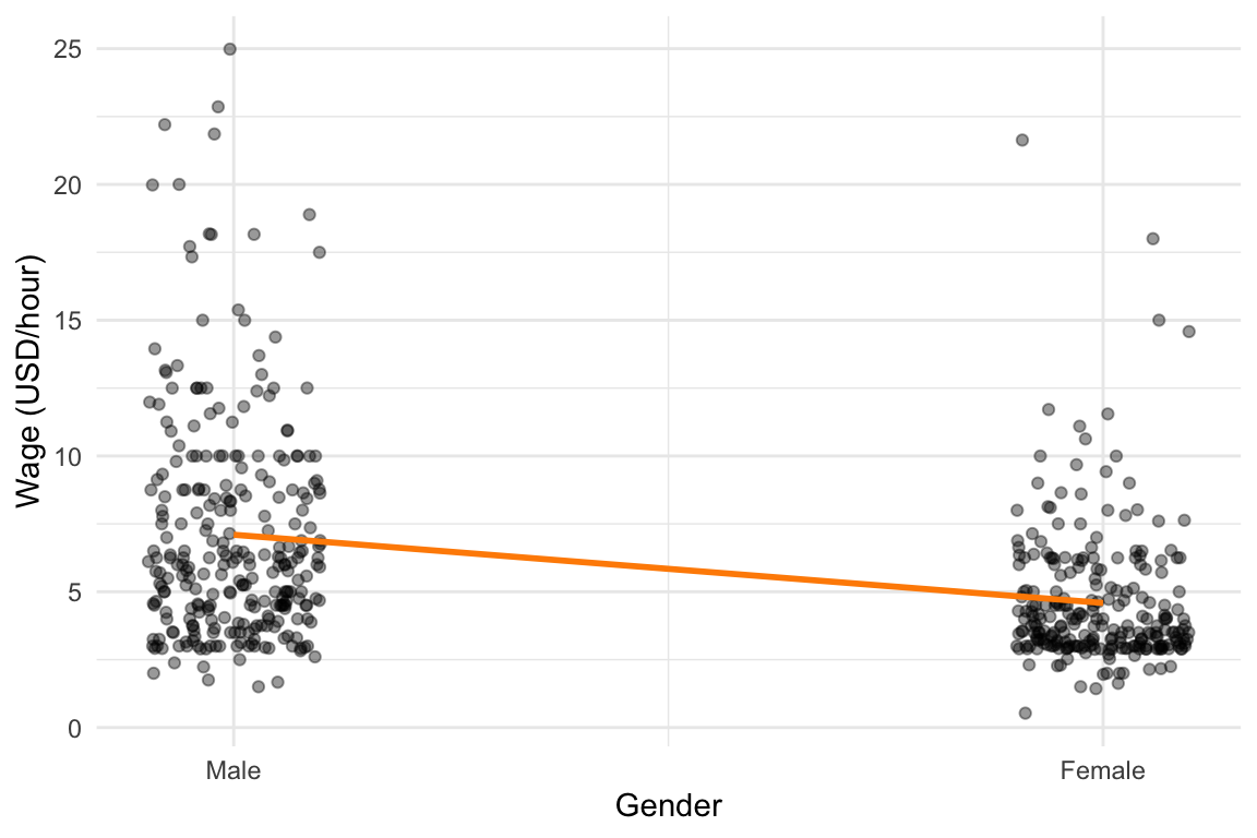
\[ \hat{y} = 7.10 - 2.51 \cdot x_1 \] as seen from output below.
Interpretation:
- The intercept (7.10) represents the average hourly wage for men (gender = 0).
- The coefficient for gender (-2.51) indicates that, on average, women earn $2.51 less per hour than men.
The overall line is visualized below:
The above model does not control for any other variables, such as education. Now, we add educ (years of education) to the model as estimate as:
\[ \hat{y} = b_0 + b_1 \cdot x_1 + b_2 \cdot x_2 \] with coefficients shown in the below output:
Call:
lm(formula = wage ~ female + educ, data = wage_data)

Residuals:
    Min      1Q  Median      3Q     Max
-5.9890 -1.8702 -0.6651  1.0447 15.4998

Coefficients:
            Estimate Std. Error t value Pr(>|t|)
(Intercept)  0.62282    0.67253   0.926    0.355
female      -2.27336    0.27904  -8.147 2.76e-15 ***
educ         0.50645    0.05039  10.051  < 2e-16 ***
---
Signif. codes:  0 '***' 0.001 '**' 0.01 '*' 0.05 '.' 0.1 ' ' 1

Residual standard error: 3.186 on 523 degrees of freedom
Multiple R-squared:  0.2588,    Adjusted R-squared:  0.256
F-statistic: 91.32 on 2 and 523 DF,  p-value: < 2.2e-16
Now, the estimated coefficient on female is -2.27, which still indicates a wage gap, but slightly smaller. This suggests that some of the wage difference was due to differences in education levels between men and women.
The interpretation of the coefficients:
- Intercept (\(b_0\)): Predicted wage for a male with 0 years of education.
- Gender (\(b_1\)): Women earn 2.27 USD less on average, holding education constant.
- Education (\(b_2\)): Each additional year of education increases expected wage by approximately the amount given by the coefficient.
To make it clear that the two gender‐specific lines share the same slope (for education) but have different intercepts, we visualize both lines given different values of the dummy (gender):
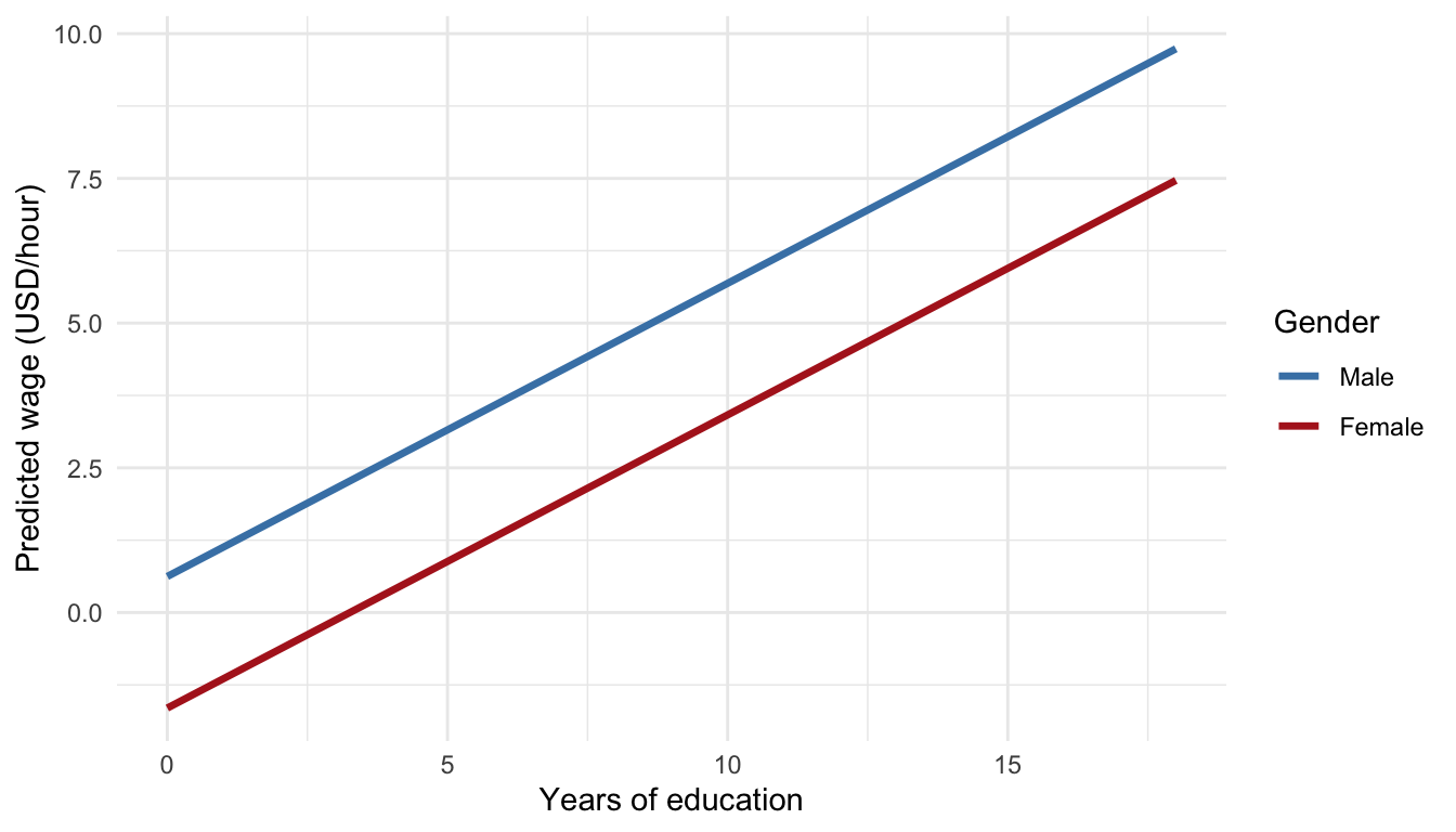
This plot illustrates two parallel regression lines; one for each group defined by the dummy variable \(x_1\). The lines are parallel because they have the same slope, but they are vertically separated because they have different intercepts. The vertical gap represents the coefficient \(b_2\), which quantifies the average difference between the two groups, after adjusting for \(x_1\).
This example demonstrates how dummy variables allow us to estimate group differences (in this case, by gender) and how those estimates change when we control for additional variables like education.
A simple model showed a gender wage gap of USD2.51/hour. After controlling for education, the gap decreased to USD2.27/hour, but remained statistically significant highlighting the value of including relevant covariates in a regression model.
30.1.3 Using Dummy Variables for Multiple Categories
In many real-world analyses, we want to compare outcomes across several distinct groups and not just two. When a categorical variable has more than two levels, we cannot capture its effects with a single dummy variable. Instead, we must create multiple dummy variables, each representing one of the non-reference categories.
Example 30.3: Wage Differences Across Gender and Marital Status
In this example, we examine how wages vary across four groups defined by the combination of gender and marital status:
- single men
- married men
- single women
- married women
To do this, we create three dummy variables, one for each group except the reference group (here, single men). This allows us to estimate how each group’s average wage differs from the base category, while controlling for education, experience, and tenure. The response is the natural logarithm of the hourly wage.
- Do married men earn more than single men?
- Are single women and married women paid differently?
- What happens to the gender wage gap once we account for experience and education?
This example showcases the flexibility of multiple regression models and how dummy variables allow us to capture meaningful differences between discrete categories in a statistically rigorous way.
Call:
lm(formula = log(wage) ~ marriedmale + marriedfemale + singlefemale +
    educ + exper + tenure, data = wage_df)

Residuals:
     Min       1Q   Median       3Q      Max
-1.95351 -0.24423 -0.04262  0.24501  1.20538

Coefficients:
               Estimate Std. Error t value Pr(>|t|)
(Intercept)    0.387817   0.102322   3.790 0.000168 ***
marriedmale    0.292091   0.055389   5.273 1.97e-07 ***
marriedfemale -0.120235   0.057984  -2.074 0.038611 *
singlefemale  -0.096750   0.057463  -1.684 0.092845 .
educ           0.083533   0.006861  12.175  < 2e-16 ***
exper          0.003164   0.001655   1.912 0.056459 .
tenure         0.015684   0.002921   5.370 1.19e-07 ***
---
Signif. codes:  0 '***' 0.001 '**' 0.01 '*' 0.05 '.' 0.1 ' ' 1

Residual standard error: 0.4058 on 519 degrees of freedom
Multiple R-squared:  0.4238,    Adjusted R-squared:  0.4172
F-statistic: 63.63 on 6 and 519 DF,  p-value: < 2.2e-16
The dummy coefficients are in log points. To express them as percentage effects we use \[ \% \text{ change} = (\mathrm{e}^{b}-1)\times 100) \]:
| Dummy | Log-coef | % change vs. single male | p-value |
|---|---|---|---|
| marriedmale | 0.292 | 33.922 | 0.000 |
| marriedfemale | -0.120 | -11.329 | 0.039 |
| singlefemale | -0.097 | -9.222 | 0.093 |
We note the following:
- Married men earn roughly 29 % more than single men with the same schooling, experience and tenure.
- Married women earn about 18 % less than single men, while single women earn roughly 10 % less.
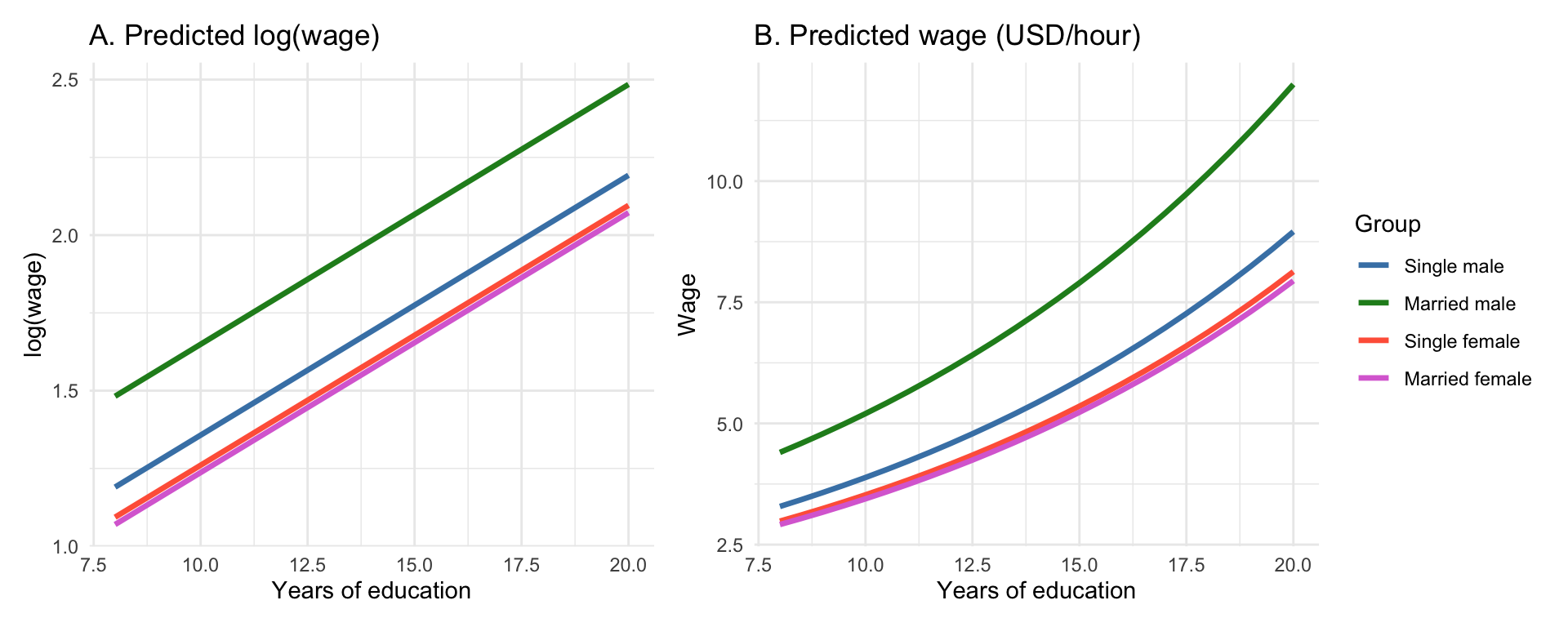
All effects are highly significant at conventional levels.
The plot below shows straight, parallel lines for the predicted log-wage and the same predictions exponentiated back to the wage scale, which appear as curved lines.
30.2 Interaction Terms in Regression
So far, we’ve allowed different intercepts in our regression models, for example, when comparing groups. But what if the slope of a variable also changes depending on the level of another variable? This is where interaction terms come into play.
In a typical multiple regression, we often assume that the effect of one explanatory variable is independent of the others. That is, the increase in \(y\) from a one-unit increase in \(x_1\) is always the same, no matter the value of \(x_2\). However, this assumption doesn’t always reflect reality. In many cases, the effect of one variable depends on another.
To capture this dependency, we include an interaction term; a product of the two variables:
\[ y = \beta_0 + \beta_1 x_1 + \beta_2 x_2 + \beta_3 (x_1 \cdot x_2) + u \]
In this model:
The effect of \(x_1\) on \(y\) changes with the value of \(x_2\): \[ \frac{\Delta y}{\Delta x_1} = \beta_1 + \beta_3 x_2 \]
Likewise, the effect of \(x_2\) on \(y\) depends on \(x_1\): \[ \frac{\Delta y}{\Delta x_2} = \beta_2 + \beta_3 x_1 \]
The coefficient \(\beta_3\) captures the interaction effect. If \(\beta_3\) is positive, then the presence of a higher \(x_2\) amplifies the effect of \(x_1\). If negative, it dampens it. Interaction terms thus allow for a more flexible model structure, where the relationship between variables can adapt depending on context.
Example 30.4: Interaction Between Education and Experience
Let’s revisit the wage1 dataset where the response is salary (\(y\)). Suppose we suspect that the return to experience (\(x_1\)) may differ depending on how many years of education (\(x_2\)) someone has. We estimate the model:
\[ \log(y) = \beta_0 + \beta_1 \cdot x_1 + \beta_2 \cdot x_2 + \beta_3 (x_1 \cdot x_2) + \varepsilon \]
If \(\beta_3 > 0\), then experience becomes more valuable as education increases.
Call:
lm(formula = log(wage) ~ educ + exper + ed_exp, data = wage1)

Residuals:
     Min       1Q   Median       3Q      Max
-2.05543 -0.29549 -0.05335  0.31047  1.44788

Coefficients:
              Estimate Std. Error t value Pr(>|t|)
(Intercept)  0.1532232  0.1673326   0.916   0.3603
educ         0.1030365  0.0127368   8.090 4.22e-15 ***
exper        0.0132641  0.0060374   2.197   0.0285 *
ed_exp      -0.0002473  0.0004945  -0.500   0.6172
---
Signif. codes:  0 '***' 0.001 '**' 0.01 '*' 0.05 '.' 0.1 ' ' 1

Residual standard error: 0.4617 on 522 degrees of freedom
Multiple R-squared:  0.2497,    Adjusted R-squared:  0.2454
F-statistic: 57.91 on 3 and 522 DF,  p-value: < 2.2e-16
Interpreting the Interaction:
- \(\beta_2\): The return to one year of experience if education is zero
- \(\beta_3\): The change in the return to experience for each additional year of education
- If \(\beta_3 > 0\), people with more schooling benefit more from each year of experience
We can visualize the interaction effect below:
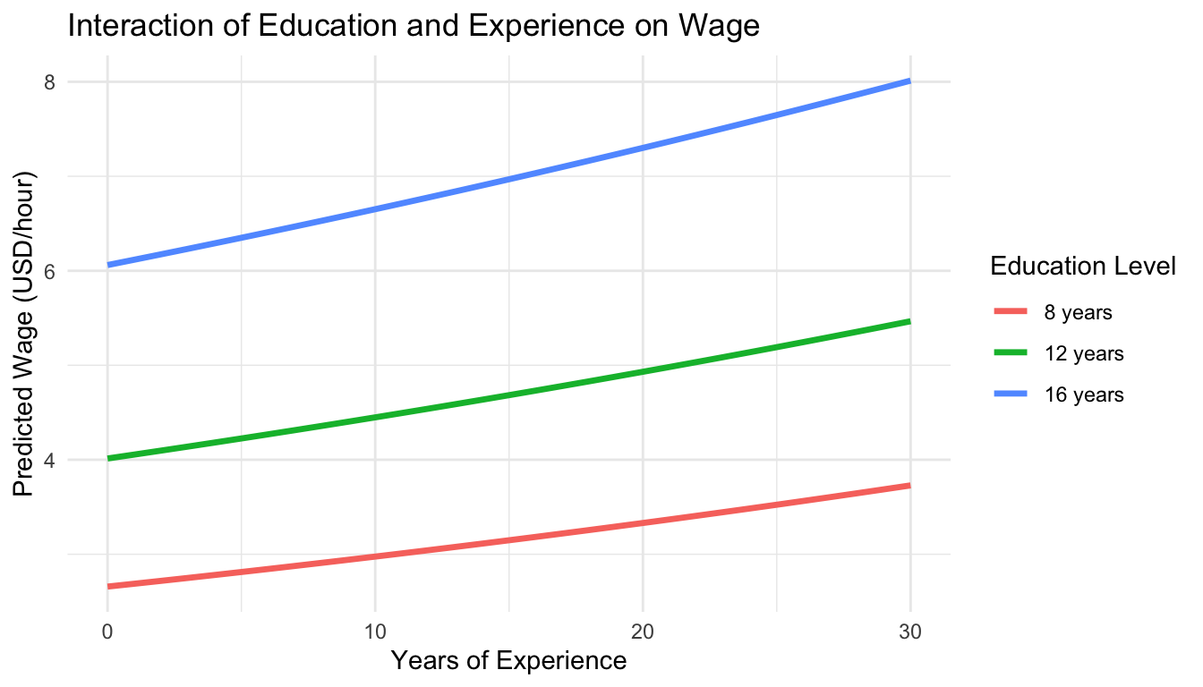
This model allows the slope of experience to vary with education. The lines in the plot diverge: people with more education experience a steeper wage growth with increasing experience, consistent with a positive interaction term.
30.3 Combining Dummy Variables and Interaction Terms
Up to this point, we’ve used dummy variables to allow for different intercepts across groups (e.g., gender or marital status). We’ve also seen how interaction terms let the effect of one variable depend on the level of another. Now we combine these ideas to build more flexible models that allow both intercepts and slopes to vary across groups.
This is especially useful when analyzing how a continuous variable like education or experience affects the outcome differently depending on group membership (e.g., male vs. female).
By including both dummy variables and interaction terms, we can:
- Estimate different intercepts across groups
- Allow the slope of a continuous variable to vary by group
- Test whether group differences in outcomes are only in levels (intercepts), or also in how the outcome responds to predictors (slopes)
Example 30.3: Wage Differences Across Gender and Marital Status (Cont’d)
Let’s consider the model:
\[ \log(y) = \beta_0 + \beta_1 \cdot x_1 + \beta_2 \cdot x_2 + \beta_3 \cdot (x_1 \cdot x_2) + \varepsilon \] where
- \(y\) is wage
- \(x_1\) is gender (0 male, 1 female)
- \(x_2\) is education
- \(x_1 \cdot x_2\) is the interaction between gender and edcuation
Moreover, we have that:
- \(\beta_0\) is the intercept for men
- \(\beta_1\) is the gender gap in intercepts (female vs. male)
- \(\beta_2\) is the return to education for men
- \(\beta_3\) is the difference in slope for women vs. men
This model allows both the starting wage and the rate of wage growth with education to differ by gender.
The model can be seen as two regressions:
- For
men(\(\text{gender} = 0\)):
\[ \log(y) = \underbrace{\beta_0}_{intercept} + \underbrace{\beta_2}_{slope} \cdot x_2 \]
- For
women(\(\text{gender} = 1\)):
\[ \log(y) = \underbrace{(\beta_0 + \beta_1)}_{intercept} + \underbrace{(\beta_2 + \beta_3)}_{slope} \cdot x_2 \]
So:
- \(\beta_1\) shows how women’s wages differ at zero education
- \(\beta_3\) shows whether the return to education is higher or lower for women
The model is fit in R and the otuput is as follows:
Call:
lm(formula = log(wage) ~ female + educ + fem_educ, data = wage1)

Residuals:
     Min       1Q   Median       3Q      Max
-2.02673 -0.27468 -0.03721  0.26221  1.34740

Coefficients:
              Estimate Std. Error t value Pr(>|t|)
(Intercept)  8.260e-01  1.181e-01   6.997 8.08e-12 ***
female      -3.601e-01  1.854e-01  -1.942   0.0527 .
educ         7.723e-02  8.988e-03   8.593  < 2e-16 ***
fem_educ    -6.409e-05  1.450e-02  -0.004   0.9965
---
Signif. codes:  0 '***' 0.001 '**' 0.01 '*' 0.05 '.' 0.1 ' ' 1

Residual standard error: 0.4459 on 522 degrees of freedom
Multiple R-squared:  0.3002,    Adjusted R-squared:  0.2962
F-statistic: 74.65 on 3 and 522 DF,  p-value: < 2.2e-16
We now plot the predicted \(\log(wage)\) for men and women across different education levels:
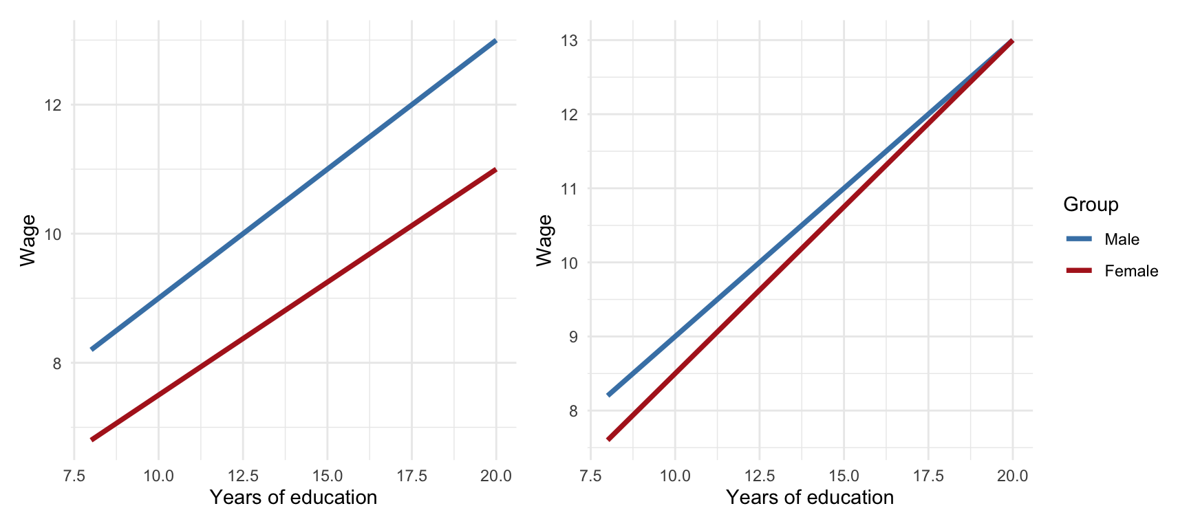
The graph displays the predicted values of log(wage) across different levels of education, separately for males and females.
- Both trend lines are upward-sloping, meaning that more years of education are associated with higher predicted log(wage) for both genders.
- The intercept for men is higher than that for women, indicating that at lower education levels, men are predicted to earn more than women.
- The slope for men is slightly steeper than that for women, suggesting that the returns to education are marginally higher for men. However, the difference in slopes is subtle and may not be easily visible to the eye.
- This difference is modeled through an interaction term between gender and education in the regression. Even when visually hard to detect, the interaction effect can be tested statistically in the regression output.
In sum, while both genders benefit from increased education, the model predicts a slightly larger benefit for men, both in starting point (intercept) and growth (slope).
Exercises
- We study how a mother’s behavior and family income affect the birth weight (in ounces) of her baby by estimating the following regression:
\[ \text{bwght} = \beta_0 + \beta_1\,\text{cigs} + \beta_2\,\text{income} + \beta_3\,\text{male} + \varepsilon \]
where:
-
bwght: birth weight in ounces, -
cigs: average number of cigarettes smoked per day during pregnancy, -
income: family income in $1,000s, -
male: a dummy variable equal to 1 if the child is male, 0 if female.
Assume the estimated equation is:
\[ \widehat{\text{bwght}} = 116.99 - 0.51 \cdot \text{cigs} + 0.09 \cdot \text{income} + 0.95 \cdot \text{male} \]
What is the effect of each additional cigarette smoked per day on birth weight?
Interpret the coefficient on
male. What does it tell us about differences in birth weight?Write the predicted birth weight equations for male and female babies.
By how many ounces is a male baby expected to weigh more (or less) than a female baby, holding other variables constant?
Solution
(a) The coefficient on cigs is -0.51, which means each additional cigarette smoked per day by the mother is associated with a 0.51-ounce decrease in birth weight, on average.
(b) The coefficient on male is 0.95, indicating that, holding smoking and income constant, male babies weigh about 0.95 ounces more than female babies on average.
(c)
For females (male = 0):
\[
\widehat{\text{bwght}} = 116.99 - 0.51 \cdot \text{cigs} + 0.09 \cdot \text{income}
\]
For males (male = 1):
\[
\widehat{\text{bwght}} = 116.99 - 0.51 \cdot \text{cigs} + 0.09 \cdot \text{income} + 0.95
\]
So the slope is the same, but males have a higher intercept.
(d) Male babies are predicted to weigh about 0.95 ounces more than females, all else equal.
- We want to explore whether the relationship between education and wages differs by gender. Consider the following estimated regression equation:
\[ \widehat{\log(\text{wage})} = 0.50 + 0.08\,\text{educ} - 0.20\,\text{female} + 0.03\,(\text{female} \times \text{educ}) \]
where:
-
educ: years of education, -
female: dummy variable (1 if female, 0 if male), -
female × educ: interaction term between gender and education.
What is the estimated return to education for men?
What is the estimated return to education for women?
What is the estimated difference in log(wage) between men and women with 12 years of education?
Does the gender wage gap increase or decrease with education? Explain using the coefficient on the interaction term.
Solution
(a) For men (female = 0), the return to education is simply the coefficient on educ:
\[
\text{Return for men} = 0.08
\]
So, for each additional year of education, men’s log(wage) increases by 0.08.
(b) For women (female = 1), the return to education is:
\[
0.08 + 0.03 = 0.11
\]
Thus, each year of education increases women’s log(wage) by 0.11 on average.
(c) The gender difference in predicted log(wage) at 12 years of education is:
\[
\Delta = -0.20 + 0.03 \cdot 12 = -0.20 + 0.36 = 0.16
\]
So, at 12 years of education, women are predicted to earn more than men (since the log-wage difference is positive).
(d) The interaction coefficient is +0.03, meaning the wage gap narrows and reverses as education increases. At low education levels, women earn less, but the gap shrinks by 0.03 in log(wage) per year of education.