23 The Chi Square Method
So far, we have focused primarily on inferential statistical methods for quantitative variables measured on interval or ratio scales, as well as binary qualitative (0-1) variables. However, in many real-world applications, we also encounter categorical variables with more than two categories (e.g., eye color, political party, type of transportation). For such qualitative variables, we need specialized methods to draw valid statistical conclusions.
This is where the Chi-Square method (\(\chi^2\)) becomes useful. The chi-square (pronounced “kai-square”) test is a non-parametric method used for hypothesis testing involving categorical data. It is particularly valuable when we are interested in understanding:
- Whether the observed distribution of a categorical variable matches an expected distribution (goodness-of-fit test Chapter 24)
- Whether there is a statistically significant association between two categorical variables (test of independence in a contingency table Chapter 25)
These tests rely on comparing observed frequencies with expected frequencies, and the test statistic follows a Chi-Square distribution under the null hypothesis. Each of these tests has its assumptions and limitations, but both are foundational tools in categorical data analysis.
23.1 The Chi-Square (\(\chi^2\)) Distribution
The chi-square (\(\chi^2\)) distribution is a probability distribution that frequently arises in statistical inference, particularly when working with categorical data. It describes a population where values are strictly non-negative. This is due to the fact that test statistics in \(\chi^2\) tests are constructed from squared deviations between observed and expected values, and squaring ensures all contributions are positive. As a result, the \(\chi^2\) distribution is bounded below by zero and only takes positive values.
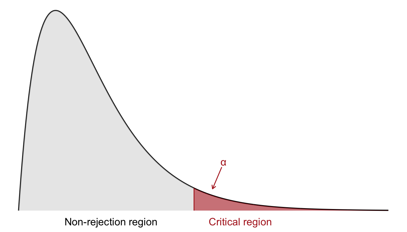
In contrast to tests based on the \(z\)- or \(t\)-distributions, which often consider both tails, the \(\chi^2\) test is typically one-sided. Since we are only concerned with whether the observed data deviate substantially from the expected frequencies under the null hypothesis, we reject the null hypothesis only for large values of the test statistic. Therefore, the critical region lies in the right-hand tail of the \(\chi^2\) distribution, as shown in Figure 23.1.
To determine the critical region, we specify a significance level \(\alpha\). The critical value is then defined such that the probability of observing a test statistic greater than this threshold (under \(H_0\)) is exactly \(\alpha\). If the observed \(\chi^2\) value exceeds this critical value, we reject the null hypothesis. As before, we determine the critical values by consulting a chi-square distribution table in Appendix C.
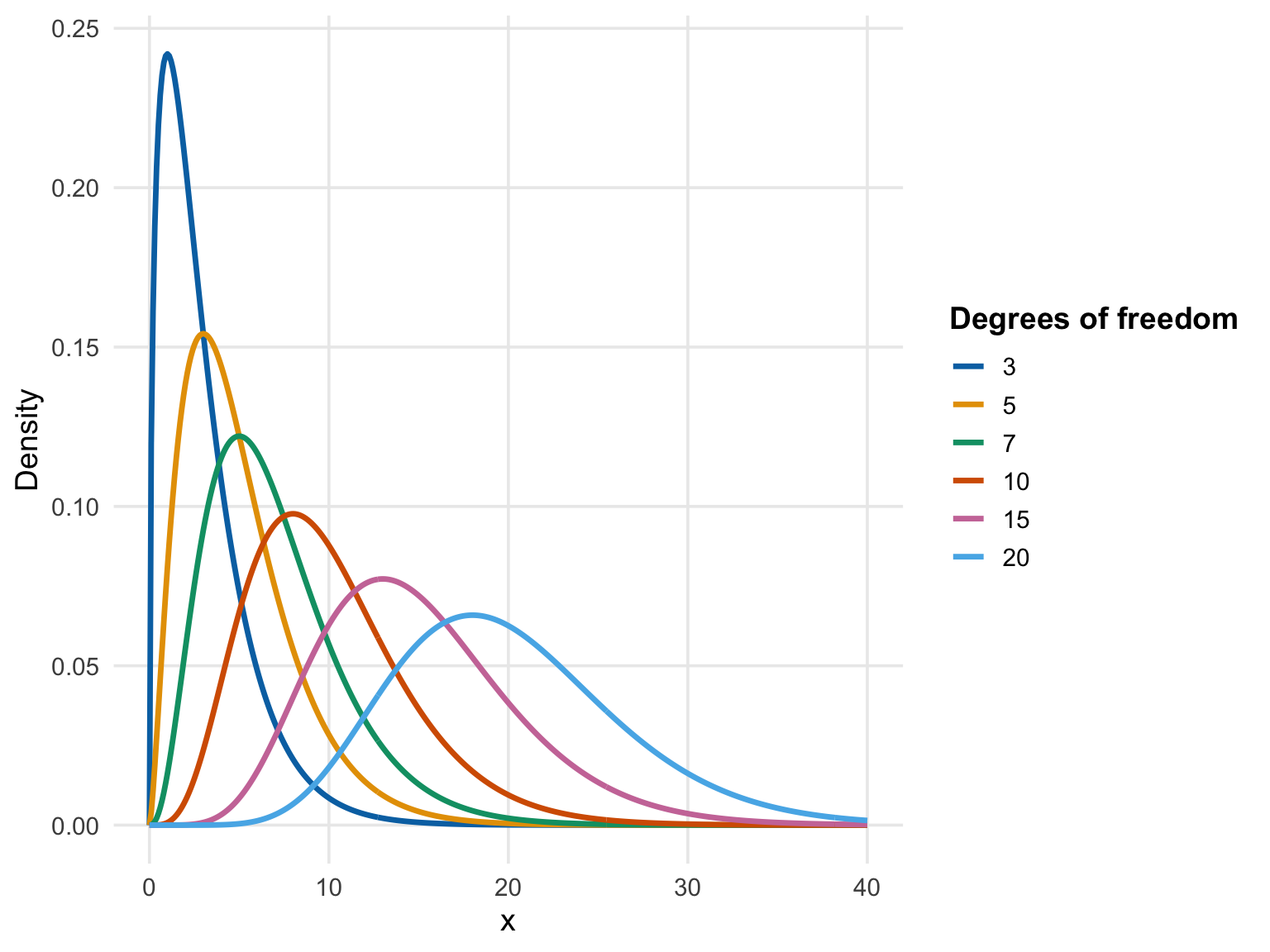
The shape of the \(\chi^2\) distribution depends on its degrees of freedom. For a small number of degrees of freedom, the distribution is heavily right-skewed. As the degrees of freedom increase, it becomes more symmetric and resembles the normal distribution. This makes the \(\chi^2\) distribution well suited for large-sample approximations. This is visualized in Figure 23.2. In the following, we will apply the \(\chi^2\) distribution to two main tests:
- The goodness-of-fit test, which assesses whether observed data match a theoretical distribution.
- The test for independence, which evaluates the association between two categorical variables in contingency tables.